4.32. LSLS: Structure factor least-squares refinement
Authors: Eric Blanc & Dieter Schwarzenbach
Contact: Eric Blanc, Institut de Cristallographie, University of Lausanne, 1015 Lausanne, Switzerland
LSLS is a least-squares refinement program that follows the recommendations of the IUCr Subcommittee on Statistical Descriptors (Schwarzenbach et al., 1989). All structural parameters may be refined, with scale, Becker & Coppens extinction, dispersion, crystal shape parameters and the volume ratio of the twins. The refinement is a full matrix refinement based on net intensities or |F|2. Restraints on distances, bond angles, dihedral angles and rigid links are included. Various weighting schemes are provided, and variances of adjusted parameters are computed according to any scheme.
4.32.1. Calculations Performed
The least-squares procedure conveniently furnishes estimators for crystallographic parameters which minimize (1)

where Yobs is an observation, such as a measured intensity, a restraint or a face distance of the crystal. Ycalc is the corresponding value computed by the model and is a function of the variables {vi}. The weights wk are in general any non-negative real numbers independent of the observations. They form a diagonal weighting matrix W.
Apart from when Ycalc is linear in the variables
{vi}, minimisation of (1) with respect to
vi leads to a system of equations which is in general not
solvable. The solution is then approximated by iterations of the linearized
problem around the nth refinement step. The vector of shifts from
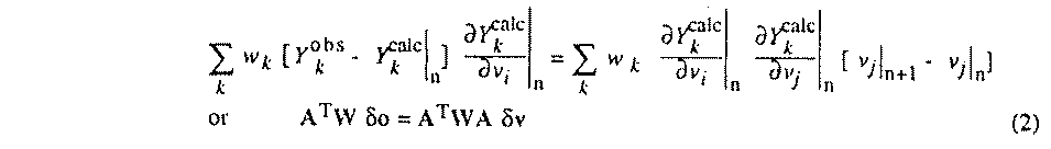
the nth to the n+1th step is given by the linear system
(2), where A is the design matrix with
Aki�=� Ykcalc/
vi
and N the normal equations matrix
N�=�ATWA.
Ykcalc/
vi
and N the normal equations matrix
N�=�ATWA.
 v�=�N-1 (ATW o)
is then an unbiased estimator of (vsolution - vn) whatever weights are chosen. It may be shown that an unbiased estimate of the variance-covariance matrix Vv of the parameters v is obtained through

by using an unbiased estimate of the variance-covariance matrix of the
observations Vo. Weights
W = Vo-1 i.e.
wk = 1/ 2 where 2 is the
variance (not an estimate) of the kth observation lead to a
minimum-variance estimate of v and Vv, and a
simplified form of (3), Vv =
N-1,
where no extra calculation is necessary to obtain Vv from
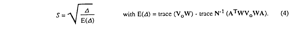
N-1. Following the recommendation of the IUCr Statistical
Descriptors Subcommittee (Schwarzenbach et al., 1988), the estimated
variance-covariance matrix of the parameters is not scaled by the global
goodness-of-fit parameter S,
2 where 2 is the
variance (not an estimate) of the kth observation lead to a
minimum-variance estimate of v and Vv, and a
simplified form of (3), Vv =
N-1,
where no extra calculation is necessary to obtain Vv from
N-1. Following the recommendation of the IUCr Statistical
Descriptors Subcommittee (Schwarzenbach et al., 1988), the estimated
variance-covariance matrix of the parameters is not scaled by the global
goodness-of-fit parameter S,
Vv is computed on the last cycle. Several types of crystallographic observations can be compared with the model: intensities Iobs, crystal shape parameters dobs and restraints Robs. Intensities are calculated by the formula

where Kk is a scale factor, Lk is the Lorentz factor of the kth reflection, and Pk its polarization factor. Tk is the transmission factor depending on the crystal shape parameters {d}, y is the Becker & Coppens extinction {e} and xi is the volume ratio of the ith twin. The real and imaginary structure factor components are given by
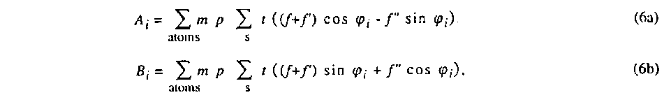
where the sum over s means over the symmetry-equivalent positions, m is
the multiplicity factor and p the population parameter, t is the
displacement factor, f is the atom form factor, f' the real part
of anomalous dispersion and f" the imaginary part of anomalous
dispersion. The angle ϕi is given by
ϕi= 2 (hix +
kiy + liz) where hi,
ki and li are the indices of the reflection
(h k l) for the ith twin.
(hix +
kiy + liz) where hi,
ki and li are the indices of the reflection
(h k l) for the ith twin.
4.32.2. General Parameters
The general parameters detailed in this section can be refined. Apart from the overall displacement factor and the scale factor(s) which are always refined unless an appropriate noref line is inserted, refinement of these parameters must be turned on in the LSLS line, and not via ref lines. Some of these parameters are tested to see if they are physically meaningful. If one parameter takes a non-physical value, the program prints a warning and either (a) stops, or (b) resets the parameter to the closest physical value, or (c) continues, depending on the user's choice.
4.32.3. Scale Factor(s)
The refined scale factor ( skf ) is not the structure scale factor commonly used in Xtal. It places the square of the structure factor on the same scale as the primary observation, such that this latter value remains untouched by any data-reduction procedure during the refinement. When sets of reflections have different scales, they can be refined separately or as a single variable. In the latter case, constraints are automatically inserted so that skf (n) = constant * skf (1).
4.32.4. Crystal Shape Parameters
The distances ( shp ) from an arbitrary origin inside the crystal to faces can be adjusted to optimize crystal shape and transmission factors. The measured values for these parameters are used as restraints,

where dkobs is the measured value for the kth distance, dkcalc is the calculated distance, which is identical to the parameter dk.
WARNING: To fix the origin of the crystal, the distances to 3 non-coplanar faces must be kept invariant. The program does not choose these faces automatically. They should be as mutually perpendicular as possible, and sufficiently large to have well-characterized Miller indices. However, when the invariant faces have been chosen, weights on these observations are automatically set to zero.
To take into account systematic errors due to magnification effect, refined distances can be constrained, or a correlation value between observations can be used. In the latter case, the variance-covariance matrix Vo is no longer diagonal, but the weighting matrix remains diagonal even in the case of 1/esd2 weights.
4.32.5. Extinction
Becker & Coppens extinction parameters can be applied or refined, either
isotropically or anisotropically. Following Zachariasen (1967), one can
distinguish two types of secondary extinction. Type I refers to crystals in
which the extinction is dominated by the mosaic distribution (described by
g), whereas effective particle size (related to the parameter
 ) is the critical parameter describing extinction in type II
crystals. For anisotropic extinction, g and become
tensorial quantities as defined according Thornley and Nelmes (1974).
) is the critical parameter describing extinction in type II
crystals. For anisotropic extinction, g and become
tensorial quantities as defined according Thornley and Nelmes (1974).
Several extinction refinement options are available: g and
can be refined separately choosing type I or type II respectively. In this
case, primary extinction is neglected. g and can also be
refined simultaneously (but only g can be tensorial) allowing primary
extinction to be taken into account. Either a Lorentzian or a Gaussian
distribution of the mosaic spread g can be selected.
A short summary of used expressions is given below. Full details can be found in Becker & Coppens (1974a, 1974b, 1975) and Zachariasen (1967).
The parameters g and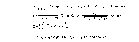
 are related respectively to the half-width of the mosaic spread distribution
 1/2
expressed in radians and to the size of the mosaic blocks
r expressed in cm by
1/2
expressed in radians and to the size of the mosaic blocks
r expressed in cm by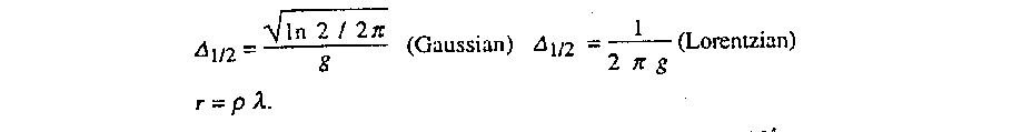
The values of g and given in the program listing are
multiplied by 104.
4.32.6. Twinning parameter(s)
(Pseudo-) merohedral twin laws may be determined automatically and entered onto the bdf by CREDUC for use by LSLS. Twin laws may also be entered directly in LSLS by use of twinop lines. By default one twin law viz. the identity operation is assumed. For centrosymmetric space groups all twin laws are generated by CREDUC or must be entered by way of twinop lines. For non-centrosymmetric space groups, each twin law generated by CREDUC or entered by way of a twinop line corresponds to a pair of twin laws: viz. the one indicated and the one related to it through a center of inversion. The two laws of the inversion-related pair in non-centrosymmetric space groups have serial numbers i and i+n where n is the number twin matrices on the bdf or twinop lines given in LSLS.
Twinning ( twi ) is treated by refining the volume fractions xi of each twin component and automatically constraining their sum to be 1.0.
For non-centrosymmetric structures, attention has to be paid to two points. Primo, anomalous dispersion should be applied. Secundo, the bdf should be prepared with each reflection and its Friedel opposite in separate packets: sepfrl on the SORTRF line.
The Becker and Coppens extinction theory used in LSLS does not take twinning into account, implying that the coupling constant between the incident and diffracted beams is forced to be symmetric under the lattice-point group symmetry.
The following example illustrates the way to handle twins in the non-centrosymmetric space group P23. CREDUC generated 2 (pairs of) twin laws:
| ( 1 0 0) | ( 1 0 0) | (-1 0 0) | |||
| ( 0 1 0) | for (1) Identity | ( 0 1 0) | and (3) Centre | ( 0 -1 0) | |
| ( 0 0 1) | ( 0 0 1) | ( 0 0 -1) | |||
| ( 0 -1 0) | ( 0 -1 0) | ( 0 1 0) | |||
| (-1 0 0) | for (2) 2-fold axis | (-1 0 0) | and (4) Mirror | ( 1 0 0) | |
| ( 0 0 1) | ( 0 0 -1) | ( 0 0 1) | |||
In order to refine only the enantiomorph-polarity parameter in this case starting with a value of 0.5, the following lines are necessary:
4.32.7. Dispersion and Neutron-Scattering-Factor Parameters
Assuming that refinement of dispersion parameters has been turned on by rd on the LSLS line, dispersion parameters can be addressed individually by re or im for the real or the imaginary parts, or as a set with dsp .
Neutron scattering factor refinement is achieved by turning on dispersion refinement and keeping imaginary parts invariant.
4.32.8. Overall Displacement Parameter
The overall displacement parameter is automatically refined if at least one atom's displacement parameter type is set to overall. It can be held invariant by using noref uov .
4.32.9. Atomic Parameters
4.32.9.1. Positional Parameters
Atomic positional parameters are always refined unless the atom is in a special position or they are explicitly constrained. noref <atom> fixes all atomic parameters of the named atom.
4.32.9.2. Displacement Parameters
The program can be used to refine overall, isotropic or anisotropic displacement parameters. In mixed mode, the displacement-parameter type of an atom is set in accordance to the value on the bdf. However it can be modified by the use of ref and noref lines. After refinement, the mode used is written on the output bdf. If the displacement factor is non-positive definite, the program will either stop ( ts ), or reset it to a positive value ( tr ), or continue with non-physical values ( tp ).
4.32.10. Invariant Parameters
ADDATM generates symmetry constraints for atoms on special positions which are written on logical record lrcons:. See the documentation of ADDATM for details.
A noref line can fix any parameter. The general form of the arguments is:
(p1/p2)(a1/a2) fixes from atomic parameter p1 to atomic parameter p2 of all atoms in list between a1 and a2 inclusive. (p1/p2) can be replaced by p1 if only one parameter is to be fixed, and a1 can replace (a1/a2) if there is only one target atom.
Atomic parameters are : x , y , z , u , u11 , u22 , u33 , u12 , u13 , u23 , pop
a1/a2 fixes all atomic parameters from atom a1 to atom a2. a1/a1 is abbreviated a1.
When an atom name is identical to an atom type name, then a1 and a2 will hold for atom types instead of individual atoms.
g1(n1/n2) fixes general parameters g1, which can be uov , skf , twi , shp , ext , dsp , re or im , from n1 to n2. If only one parameter is kept invariant, n1 can be used for n1/n2.
For dispersion refinement, dsp fixes real and imaginary parts and it is equivalent to ( re / im ).
The syntax of the ref line is identical to that of noref. When mixed displacement mode has been selected on the LSLS line, ref/noref lines can be used to change atomic displacement types. ref U converts the displacement type to isotropic, while ref U11/U23 set the displacement type to anisotropic.
These examples show how to set to isotropic the displacement parameter type for all 6 nitrogen atoms, except for atom N2. There is a difference in the resulting displacement parameters values between these two examples. In the first example, all nitrogens are first changed to isotropic, and then the displacement factor of atom N2 is reset to an anisotropic tensor. In the second example, the displacement parameter of atom N2 is not changed at all.
WARNING If atom types Y and U appear in the atom type list, atomic parameters y and& u must be lowercase.
4.32.11. Constrained Parameters
As for invariant parameters, symmetry constraints are read from the input bdf logical record lrcons:. Linear constraints between parameters can also by introduced by constr lines :
| p = Q + f(1)*r(1) + ... + f(n)*r(n) where : | |
| p = object (dependent) parameter (same format as ref/noref lines) | |
| Q = constant term | |
| f(i) = ith multiplicative term | |
| r(i) = ith reference (independent) parameter (same format as ref/noref lines). |
WARNING Origin fixing is carried out by shift-limiting restraints, following the algorithm of Flack & Schwarzenbach (1988). Additional constraints should not be used in LSLS in polar space-groups.
The normal-equations matrix is constructed for independent variables only to minimize storage size and inversion time. The constraints modify the derivative vector, which leads to an unconstrained least-squares problem. The dependent parameters po contribute to the derivatives vector of the reference parameters pr, which become:
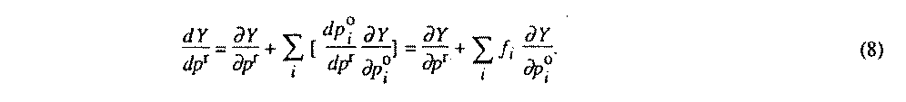
The dependent parameter estimated standard deviation is then given by (9) :

4.32.12. Restraints
Restraints  are additional stereochemical pseudo-observations used
to restrict interatomic geometry. For a discussion of the relations between
rigid bodies and restraints, see Didisheim & Schwarzenbach (1987).
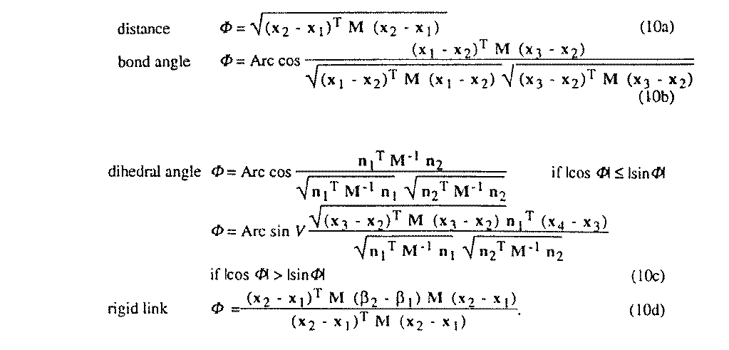
Distance, bond-angle, dihedral-angle and rigid-bond restraints are provided. If
M and M-1 are respectively the direct and
reciprocal
metric tensors, xi is the position of atom i expressed
in the crystal coordinates,
are additional stereochemical pseudo-observations used
to restrict interatomic geometry. For a discussion of the relations between
rigid bodies and restraints, see Didisheim & Schwarzenbach (1987).
Distance, bond-angle, dihedral-angle and rigid-bond restraints are provided. If
M and M-1 are respectively the direct and
reciprocal
metric tensors, xi is the position of atom i expressed
in the crystal coordinates,  i the displacement tensor of atom
i expressed in the
same basis, n1 = (x2 -
x1) ^ (x3 - x2),
n2 = (x3 - x2) ^
(x4 - x3) and V the volume of the
cell, then restraints are given by (10) :
i the displacement tensor of atom
i expressed in the
same basis, n1 = (x2 -
x1) ^ (x3 - x2),
n2 = (x3 - x2) ^
(x4 - x3) and V the volume of the
cell, then restraints are given by (10) :
When the normal-equations matrix is ill-defined, it is possible to force it into a positive-definite form, which is easily invertible. The usual way to do this is to use shift-limiting restraints which increase the diagonal element Nii of the variable vi leading to the degeneracy. Two possibilities are available in LSLS: (a) when the weight w of the restraint is greater than 1, the restraint equation adds the quantity w(viobs - vicalc)2 to the minimized function (1), so the diagonal element becomes Nii + w. This type of shift-limiting restraint may then be viewed as a pseudo-observation whose value is taken to be the variable's value in cycle n, and the restraint imposes that vi in cycle n+1 should be "close to" its former value. (b) If w is smaller than 1, it is interpreted as a Levenberg-Marquardt parameter (see Press, Flannery, Teukolsky & Vettering (1986)). There is no pseudo-observational justification to this method where the diagonal element is multiplied by a w independent of the Nii. It should be pointed out that tests to determine the optimal Levenberg-Marquardt parameter are not carried out by LSLS.
4.32.13. Weights
LSLS provides 3 different weighting schemes: the usual minimal variance w = 1/esd2, unit weights w = 1, or weights read from the bdf (idn 1900 is taken as the square root of the weight on Y); this latter possibility allows the user to define his/her own weighting scheme. In any case, the goodness of fit and the parameter variance-covariance matrix are computed according to (3) and (4).
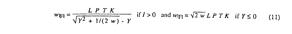
Weights on |F| are computed from weights on the refined quantity Y (either |F|2 or I) by (11) where LPT is set to 1.0 if Y = |F|2. These |F| weights are used in the calculation of the weighted R-factor.
4.32.14. Reflection Classification
A reflection can be omitted from the refinement under several conditions: if it is flagged as suffering form extinction (rcode 3), if its weight is 0, if its weighted difference w1/2 |Yobs - Ycalc| is greater than some user defined value, or if Y/esdY is less than a user defined threshold. These unused reflections do not contribute to the matrices, Durbin-Watson statistic, and goodness-of-fit. Less-than reflections are those for which Y/esdY less than the cutoff value, and those with rcode = 2. In the latter case, the reflections are discarded only if Yobs is greater than or equal to Ycalc. The status code is never updated by LSLS.
The meaning of the printed status codes is the following: F is for reflections without their Friedel mate, A is for systematically absent reflections. Reflections flagged with these codes are always used in the refinement. E is for a reflection suffering from extinction, L for less-than reflections, i.e. which Y/esdY smaller than the threshold, W for reflections with a weight of zero, and R for a rejected reflection for which w1/2 | Yobs -Ycalc| is greater than the cutoff. Reflections marked with these codes are always excluded from the refinement. U is for unobserved reflections; it corresponds to rcode = 2. The asterisk * marks reflections which do not contribute to the matrix.
4.32.15. R-Factors
The unweighted and weighted R-factors are printed by the program. The unweighted R-factor is defined as:

and the weighted R-factor by:

For the 4 R-factors printed by the program:
(1) marked "Of contributing reflections" is calculated with R, Y = |F| and M = NREF.
(2) marked "Of weighted contributing reflections" is calculated with wR, Y = |F| and M = NREF.
(3) marked "Of Observations" is calculated with R; for refinement on |F|2, Y = |F|2; for refinement on I, Y = I; and M = NOBS.
(4) marked "Of Weighted Observations" is calculated with wR; for refinement on |F|2, Y = |F|2; for refinement on I, Y = I; and M = NOBS.
4.32.16. File Assignments
Reads parameter- and observation- information from the input archive bdf
Writes refined parameters on output archive bdf
Optionally writes variance-covariance matrix to file cmx
Optionally writes parameters to file pch
4.32.17. Examples
title Gd3Ru4Al12 compid gra CIFENT cifin STARTX upd sgname -P 6C 2C REFCAL neti inst 1 excl LSABS ADDATM extinc typ1 is gaus 0.005 atom Al1 0.1622 0.3244 0.5763 0.008 atom Gd 0.1928 0.3856 0.25 0.007 atom Ru1 0.5 0 0 0.007 atom Al3 0.3333 0.6667 0.0119 0.008 atom Al4 0 0 0.25 0.008 atom Ru2 0 0 0 0.007 atom Al2 0.5637 0.1274 0.25 0.008 0.95 atom Ru3 0.5637 0.1274 0.25 0.008 0.05 LSLS cy 5 ad ax pp tr rs sm noref shp(1) shp(3) shp(5) noref pop ref pop(Ru3) pop(Al2) constr x(Ru3)=0.0+1.0*x(Al2) constr u(Ru3)=0.0+1.0*u(Al2) constr pop(Ru3)=1.0-1.0*pop(Al2) REGFE sr 1 nan tab finish |
To refine the crystal shape, the absorption program LSABS is run just after the conversion from raw data to net intensities. No averaging is done, and the refinement is made on all intensities. 3 faces are kept invariant. Ru3 and Al2 are constrained to the same position, and the same displacement parameter. The stereochemical disorder of these atoms is taken into account constraining the total population of the site to be equal to 1. The variance-covariance matrix is saved to be used in the calculation of distances by REGFE.
compid coanp CIFENT cifin STARTX upd latice n p symtry x,y,z symtry -x,y,1/2+z symtry -x,1/2+y,-z symtry x,1/2+y,1/2-z NEWCEL transf 0 0 1 1 0 0 0 1 0 CREDUC REFCAL excl fsqr ffac SORTRF ord lkh aver 1 sepfrl f2rl ADDATM Atomic parameters omitted here for brevity LSLS cy 1 f2 cs 3.0 noref C N O H LSLS cy 5 f2 cs 3.0 rp ep FOURR MAPLST finish |
In this example, the space group is changed by NEWCEL, then twins are searched (CREDUC), the data are converted to |F|2 and averaged in separate packet for Friedel pairs. The scale factor is refined alone for one cycle, and then all structural parameters are refined, including enantiomorph (absolute structure) parameter. When the initial value of the scale factor is far from the real one, it can be useful to refine the scale factor alone in a first refinement step.
4.32.18. References
Becker, P.J. & Coppens, P. (1974). Acta Cryst. A30, 129-147.
Becker, P.J. & Coppens, P. (1974). Acta Cryst. A30, 148-153.
Becker, P.J. & Coppens, P. (1975). Acta Cryst. A31, 417-425.
Bernardinelli, G. & Flack, H.D. (1985). Acta Cryst. A41, 500-511.
Didisheim, J.-J. & Schwarzenbach, D. (1987). Acta Cryst. A43, 226-232.
Flack, H.D. (1983). Acta Cryst. A39, 876-881.
Flack, H.D. & Schwarzenbach, D. (1988). Acta Cryst. A44, 499-506.
Press, W.H., Flannery, B.P., Teukolsky, S.A. & Vetterling, W.T. (1986). Numerical Recipes. Cambridge University Press. Cambridge.
Thornley, F.R. & Nelmes, R.J. (1974). Acta Cryst. A30, 748-757.
Schwarzenbach, D. et al. (1989). Acta Cryst. A45, 63-75.
Zachariasen, W.H. (1967). Acta Cryst. 23, 558-564.