Teaching crystallographic and magnetic point group symmetry using three-dimensional rendered visualizations

Marc De Graef

1. Abstract

Direct visualization of crystallographic and magnetic point group symmetry by means of computer graphics substantially simplifies the teaching of point group symmetry at the undergraduate and graduate levels. A method is proposed for the creation of still images and animated movies for all 32 crystallographic point groups, and for the 122 magnetic point groups. For each point group, the action of the symmetry operators on scalar and pseudo-scalar objects, as well as polar and axial vectors, is represented as a three-dimensional rendered (ray-traced) image. All images and movies are made available as supplementary educational material via a dedicated web site.

2. Introduction

Symmetry is of fundamental importance to many branches of science. While the concept of symmetry was well known to the Greek philosophers, it was not until the early nineteenth century that the basic notion of a group and the machinery of group theory were developed by Evariste Galois (1811-1832). Galois used the symmetry properties of n-th order polynomial equations to decide whether or not the solutions can be written down using rational functions and n-th order roots; in particular, he showed (see [Livio(2005)] for an entertaining account) from the symmetry of the quintic equation that its solution can not be written down using only standard mathematical operations (additions, subtractions, multiplications, divisions, and roots). Today, group theory occupies a central place in both modern and classical physics, in chemistry, and in material science and engineering.

In this contribution, we will focus on the symmetry of 3-D crystals, in particular on the 32 crystallographic point groups, and the 122 magnetic point groups. When teaching a crystallography course to a group of students, in particular at the undergraduate level, it is not always easy to convey the meaning of the concept of a group. The mathematical definition of a group is not difficult per se, but is often presented in a rather abstract way, and, at first, can appear to be unrelated to anything tangible. Some text books refer to infinite sets of numbers combined with basic arithmetic operators to illustrate what groups are and how they work; others use the Cayley square and low order groups, such as the permutation groups, to illustrate what a group is.

Individual symmetry elements can be represented readily by simple drawings, and many textbooks offer very clear drawings of rotation axes, mirror planes and so on (e.g. [Burns and Glazer(1990),McKie and McKie(1986)]). For crystallographic point groups, one usually resorts to graphical representations by means of stereographic projections to illustrate the structure of each group. While this is accepted practice (after all, the International Tables for Crystallography, Volume A, [Hahn(1996)] lists all crystallographic point groups by means of their stereographic projections), that does not mean that these representations are easily grasped by beginning students. Consider what is involved in this representation: the student is asked to interpret a 2-D stereographic projection (which itself is not as simple as the more familiar orthogonal and perspective projections) of an abstract 3-D object (the point group), and to reconstruct from this projection what a 3-D object with the corresponding symmetry might look like. Should we be surprised, then, to find that many students have a difficult time with stereographic projections of point groups?

Not everyone has the ability to perform mental operations, such as rotations, on 3-D objects without actually touching them or observing them in 3-D [De Graef(1998)]. And yet, the very definition of symmetry operations involves the concept of motion of an object: an object has a symmetry property when it can be brought into self-coincidence by an isometric motion (i.e., by a translation, rotation, mirror, or inversion operation). It is not a trivial matter to execute such motions by pure thought alone. Research into the way the human brain interprets 3-D visual cues indicates that there are two different levels at which this information can be processed. If 3-D information is presented in 2-D, then the brain has to perform a cognitive effort to convert the information to a 3-D representation. Different people have different approaches to this conversion, and not everyone can easily perform this task. On the other hand, if the information is presented in true 3-D form, then the human brain, which is highly capable of 3-D perception, does not need to use its congnitive centers to convert the information; all cognitive efforts can go towards interpreting and understanding the meaning of the 3-D object itself.

We would substantially simplify the student's task if we could eliminate one or more intermediate steps in the representation of point groups. Since a point group represents a 3-D object, why not directly visualize the point group in 3-D, using computer graphics and animation? Once the 3-D representation is understood, the corresponding stereographic projection should pose no substantial problems [De Graef(1998)]; indeed, an understanding of the 3-D nature of point groups may even help to understand the stereographic projection itself.

In this article, we refer to symmetry in its original meaning, namely invariance under spatial geometric transformations, such as rotations, and reflections. In addition, we also consider time reversal symmetry, as it pertains to the magnetization state of an object. We restrict the discussion to the domain of classical physics. In section 3, we describe how the 32 crystallographic point groups can be represented graphically by means of computer-generated 3-D drawings. Then we introduce the notion of time reversal symmetry, first by means of a mathematical representation, and then by means of a graphical color coded 3-D rendering. High resolution images and movies are available from a dedicated web site: http://mpg.web.cmu.edu. We will refer to this web site as supplemental material. The visualizations of the 32 crystallographic point groups in this paper have been used for the past decade in an undergraduate crystallography course at Carnegie Mellon University (Department of Materials Science and Engineering); the magnetic point group representations were added to this course during the past year.

3. Visualizing the 32 crystallographic point groups

The symmetry elements that make up the 32 crystallographic point groups belong to two classes: Type I elements are rotations (and, in the case of space groups, lattice translations) which do not change the handedness of an object, and Type II elements include mirrors and the inversion operator, which do change the handedness.

We will represent symmetry operators graphically as illustrated in Fig. 1, which shows the symbols for rotation axes of orders 2, 3, 4 and 6, the inversion, and a mirror plane. The rotation axes are represented as cylindrical rods with polygonal end-caps reflecting the order of the rotation axis. The mirror plane is represented as a rectangular plane, with a reflective surface property. All 3-D renderings presented in this paper were created with the rayshade program [ray()], a public domain ray tracing package. It is not difficult to convert the rayshade input files to a format suitable for other rendering programs, such as the popular PoV-Ray package [pov()]. All ray tracing input files are available as part of the supplementary material for this paper.

**Figure 1:** Illustration of the graphical representation of symmetry elements. From left to right: rotation axes of order 2, 3, 4 and 6; an inversion center; and, towards the rear, a mirror plane.

Note that the handedness of an object is an arbitrary property, in the sense that there is no absolute property of 'right-handedness'. In fact, the usual terminology of left-handed/right-handed or clockwise/counterclockwise is only a convention based on the anatomy of the human body or on the arbitrary historical fact that the hands of a clock run, well, clockwise. While handedness is arbitrary, the act of changing the handedness of an object can be described unambiguously by means of coordinate transformations. We will adopt the active view of coordinate transformations, which means that a symmetry operation will be considered to change (i.e., rotate, invert, or mirror) the object while leaving the reference frame unchanged.

As an example, we will consider the crystallographic point group 2/m (in the international or Hermann-Mauguin notation; in the alternative Schœnflies notation the symbol would be C_2h). This point group consists of a two-fold rotation axis, 2, which we take to lie along the z-axis of a cartesian reference frame; a mirror plane, m, normal to the two-fold axis; and an inversion center, i, located at the origin. When we take these three elements along with the identity operator, E, we can easily show that the set {E, 2, m, i} satisfies all the conditions for a group. Each symmetry operation can be represented mathematically by a $3\times 3$ transformation matrix M:

$\displaystyle M(E) = \left(\begin{array}{ccc} 1 & 0 & 0 \\ 0 & 1 & 0\\ 0 &... ...\begin{array}{ccc} -1 & 0 & 0 \\ 0 & -1 & 0\\ 0 & 0 & 1\end{array}\right);$
$\displaystyle M(m) = \left(\begin{array}{ccc} 1 & 0 & 0 \\ 0 & 1 & 0\\ 0 &... ...begin{array}{ccc} -1 & 0 & 0 \\ 0 & -1 & 0\\ 0 & 0 & -1\end{array}\right).$			(1)

The matrix M(2) transforms a point with coordinates (x, y, z)^T to the point (-x, -y, z)^T, where T stands for the transposition operator, i.e., we write position vectors as column vectors. We define the parity, p, of an operator, O, as the determinant of the representing matrix, i.e.:

$\displaystyle p_{O} \equiv \det\vert M(O)\vert.$

(2)

Two of the operators of 2/m have even parity, the other two have odd parity:

$\displaystyle p_{E} = 1; \quad p_{2} = 1; \quad p_{m} = -1; \quad p_{i} = -1.$

(3)

An operator of odd parity changes the handedness of the object on which it operates; in other words, an operator of odd parity is a Type II operator. We will refer to the parity of a Type I or Type II operator as the spatial parity, to distinguish it from the temporal parity which will be defined in section 5.

**Figure 2:** Rendered representation of the point group **2/m**: (a) shows just the symmetry elements, along with the blue lines which represent the cartesian coordinate axes; in (b), the blue spheres represent scalar objects, whereas the object in (c) is a pseudo-scalar object, i.e., it has handedness.

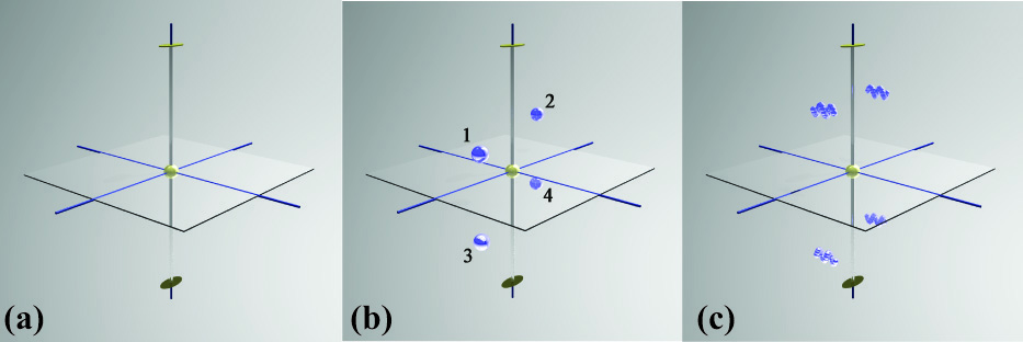It is now straightforward to create a graphical representation of the point group 2/m, by placing the building blocks of Fig. 1 in the correct relative position and orientation. The resulting representation is shown in Fig.2(a). The blue lines represent the axes of the cartesian reference frame. It is not difficult to repeat this procedure for all 32 crystallographic point groups; the resulting renderings are available as $1200\times 1200$ pixel JPEG images in the supplementary material. The file names are chosen to be easily readable; for the point group 2/m the file is called raw_2overm.jpg, whereas the point group $\mathbf{\bar{3}m}$ $(\mathit{D}_{3d})$ can be found in the file raw_bar3m.jpg, and so on. The prefix raw_ refers to the fact that only the point group symmetry operators are represented; no objects are present in these renderings.

We can enrich the graphical representation of the point groups by adding an object and all its equivalent images. In principle, we can add any kind of object (even mathematical abstract objects, such as a second rank symmetric tensor represented by an oriented ellipsoid), and determine how the symmetry elements of the point group would copy this object into equivalent positions and orientations. The simplest object is one that does not have any handedness nor preferential direction, i.e., a sphere. As shown in Fig. 2(b), if we place a sphere at the location (x, y, z)^T (labeled as point 1), then there will be equivalent spheres at the positions (-x, -y, z)^T (2), (x, y, -z)^T (3), and (-x, -y, -z)^T (4). The spheres represent scalar objects, because there is no handedness nor directionality involved.

If we replace the sphere by an object with handedness, then we obtain the representation in Fig. 2(c). The object is a helix consisting of smaller spheres. The helix has both handedness and an orientation in space; if we consider only the handedness for now, then the helix is a representation of a pseudo-scalar object, i.e., there are two versions of the object, a left-handed and a right-handed helix. The helices at positions (1) and (2) (referring to Fig. 2(b)) have the same handedness, since they are related to each other by a symmetry operator (the two-fold axis 2) of even spatial parity (). The other two helices, at positions (3) and (4), have opposite spatial parity with respect to the one at position (1), since they are generated by symmetry operators of odd spatial parity, m and i.

**Figure 3:** Stereographic projections for scalar objects (a and c) and pseudo-scalar objects (b and d) for the point groups **2/m** (a and b) and $\mathbf{m\bar{3}m}$ (c and d). Red points have opposite handedness from black points; filled circles correspond to the Northern hemisphere, open circles to the Southern hemisphere.

**Figure 4:** 3-D rendered representation of the cubic point group $\mathbf{m\bar{3}m}$ using a helical object.

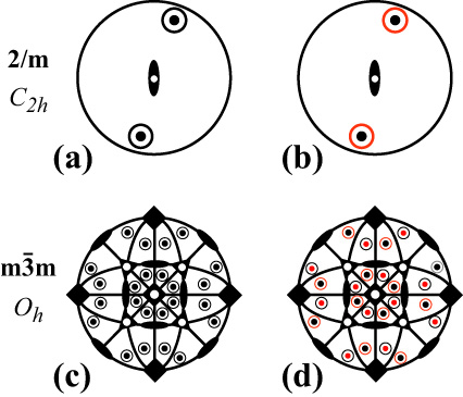
In the standard stereographic projections of the point groups, one usually only deals with scalar objects, as shown in Fig. 3(a). Filled black circles correspond to points in the Northern hemisphere, whereas open circles represent points in the Southern hemisphere. Pseudo-scalar objects can be included by color-coding the projection points. Fig. 3(b) shows the same point group but with the odd parity equivalent points colored in red. Similar projections for the highest order cubic point group $\mathbf{m\bar{3}m}$ (O_h) are shown in Fig. 3(c) and (d). It is clear that the higher the point group order, the more complex the stereographic projection becomes, and the harder it is to visualize the symmetry in 3-D. Fig. 4 shows the corresponding 3-D rendered representation for $\mathbf{m\bar{3}m}$ , using a pseudo-scalar object (helix). Equivalent helices occur in two sets of three around the three-fold rotation axis near the center of the image; three of the helices are right-handed, the other three are left-handed. This set of six helices is then copied by the vertical four-fold axis to three other locations, and by the horizontal mirror plane to four locations in the lower half of the representation, for a total of 48 equivalent positions.

In the supplemental material, the reader will find point group renderings for all 32 crystallographic point groups employing a scalar object (file names starting with the prefix scalar_) and a pseudo-scalar object (file names starting with the prefix pseudoscalar_). In addition, animations are available in which the entire point group object rotates around the vertical axis, to facilitate interpretation of the various symmetry elements and their relative orientations.

The 3-D rendering approach can also be used to illustrate the concept of special positions, i.e., positions that coincide with one or more symmetry elements. Consider the point group 4/mmm; this group of order 16 consists of a fourfold axis with a perpendicular mirror plane, four mirror planes that contain the fourfold axis, four twofold axis and the inversion operator. Fig. 5 shows six frames of an animation (available as the file special_positions.mpg in the supplemental material). In frame (c), all spheres are located at general positions (with multiplicity 16); the spheres approach the diagonal mirror planes and when they lie on the mirror planes (d) the number of sphere positions is reduced by a factor of two, reflecting the fact that the special positions have a lower multiplicity than the general position. In Fig. 5(e) the spheres approach the horizontal mirror plane; when they reach the plane (f), the multiplicity decreases again by a factor of 2. Starting from (c), the points approach the fourfold axis (b), and when they coincide with the axis, the multiplicity of the resulting special position is reduced to 2.

**Figure 5:** 3-D rendered representations of the general equivalent positions of the point group **4/mmm** (c); in (d), the points approach the diagonal mirror plane, and in (e) they coincide with the mirror plane, resulting in special positions with a multiplicity that equals half of the group order. In (f), the special points lie at the intersection of two mirror planes, halving the multiplicity once more. Starting from (c), the points approach the vertical axis (b) until they coincide with it in (a) to result in a multiplicity of 2.

4. Polar and axial vectors

One can easily extend this method of graphical representations to other objects, such as vectors (which can be represented by arrows), symmetric second rank tensors (representable by a general ellipsoid), and so on. In this section, we will consider the effect of crystallographic symmetry on vector objects. There are two types of vectors: polar vectors and axial vectors. We know from basic physics that moving electrical charges generate a magnetic field. In particular, electrons moving around the nucleus of an atom generate tiny electrical currents which give rise to a vector quantity known as the magnetic moment. The magnetic moment is represented by the vector $\bm{\mu}$ ; the magnitude of this vector is equal to the current multiplied by the area of the circular orbit of radius r, i.e.,

$\displaystyle \vert\bm{\mu}\vert = I\pi r^{2}.$

(4)

The direction of the moment vector is determined by the direction of the current; for a counter-clockwise current (Fig. 6(a)), the moment vector points up, whereas for a clockwise current (Fig. 6(b)) the moment points down.

**Figure 6:** Representation of an axial vector resulting from a counter-clockwise electrical current (a) and a clockwise current (b). (c) shows an electrical dipole moment vector. In (d), it is shown that the mirror image of an axial vector that is parallel to the mirror plane points in the direction opposite to that of the original vector.

If we consider the electrostatic equivalent, the polarization vector p, then the situation is different, since the electrostatic dipole moment is defined as the charge, q, multiplied by the separation, d, between the negative and positive charges (Fig. 6(c)). The image of a polar vector parallel to a mirror plane is a new vector with the same direction as the original one. For an axial vector, on the other hand, (Fig. 6(d)) a counter-clockwise current becomes a clockwise current when viewed in a mirror, so that the mirror image of a magnetic moment vector parallel to a mirror plane is a moment vector parallel to the original one, but pointing in the opposite direction.

Polar and axial vectors can be defined formally by the transformation rules they obey. Consider a symmetry operator O described by the $3\times 3$ matrix M_ij. A polar vector p is then defined as a first-rank tensor which satisfies the following transformation rule (with summation over repeated indices implied; the asterisk indicates the new reference frame):

$\displaystyle p^{\ast}_i = M_{ij} p_j$ (polar).

(5)

For an axial (or pseudo-) vector, $\bm{\mu}$ , we must multiply this expression by the determinant of the transformation matrix:

$\displaystyle \mu^{\ast}_i = \det\vert M\vert M_{ij}\mu_j$ (axial).

(6)

In other words, for a Type II operation, an axial vector undergoes an additional sign change. Alternatively, we can use the parity of the operator O:

$\displaystyle \mu^{\ast}_i = p_O M_{ij} \mu_j.$

(7)

Let us analyze the meaning of these transformation rules by means of a graphical example. Consider a single mirror plane, m, oriented normal to the z-axis through the origin (see Fig. 7). A polar vector p has components $[0,\sin\theta,\cos\theta]$ where $\theta=0..90^{\circ}$ , i.e., the vector is oriented parallel to z when $\theta=0^{\circ}$ and is parallel to the mirror plane when $\theta=90^{\circ}$ . Let us also assume that this vector is located at the point with coordinates r = (0, 0, 1). The transformation of a vector under the point symmetry operation m then consists of two steps: first, compute the image of r under m, which is (0, 0, -1). Then move the vector p from (0, 0, 1) to the origin, apply equation (5), and move the resulting vector to the point (0, 0, -1).

To enrich the graphical representation of these transformations, we will use a color subtraction code. The original vector p is represented by a white vector, i.e., with red-green-blue components [R, G, B]=[1, 1, 1]. The image of p under an operator with even parity will also be represented as a white vector. For operators with odd spatial parity, we will remove one of the colors, say green, so that the image of p under an operator with odd spatial parity has colors [1, 0, 1] (magenta). In the next section, we will extend this code by removing the color red in the presence of anti-symmetry. From here on, we will represent all regular symmetry elements (Types I and II) by dark blue graphical symbols.

Fig. 7 shows how a polar and an axial vector transform under the action of a single mirror plane m. For the axial vector, the mirror image must be inverted due to the fact that p_m = -1 in equation (7). This leads to the somewhat counter-intuitive result that the image of an axial vector parallel to a mirror plane points in the direction opposite to the original vector, whereas the image of an axial vector normal to a mirror plane points in the same direction.

**Figure 7:** Representation of the action of a mirror plane m on a polar vector and an axial vector. The original vectors are rendered in white, whereas vectors related to the original ones by a Type II symmetry operation (odd spatial parity) are rendered in purple.

5. Time reversal symmetry

In this section, we consider the effect of time reversal, and we propose a graphical method to represent the operation of symmetry elements with a time reversal component. If we consider the definition of the magnetic moment in the previous section, we can rewrite equation (4) as

$\displaystyle \vert\mu\vert = \frac{\mathrm{d}q}{\mathrm{d}t}\pi r^{2}.$

(8)

It is clear that a reversal of time changes the sign of the current and, hence, reverses the direction of the magnetic moment vector $\bm{\mu}$ . For a polar vector, time reversal has no effect at all. We will represent the operation of time reversal by the operator R. When we combine the time reversal operator with a regular symmetry operator, O, we will denote the new operator by a primed symbol, O'. Primed symmetry operators are known as anti-symmetry operators, and they are formally represented by the product of a regular symmetry operator with the time reversal operator;

$\displaystyle O' = OR= RO.$

(9)

Note that, since there is no mixing of spatial coordinates and the time coordinate, the two operators always commute.

**Figure 8:** Representation of the operations of the point group **2/m** on an axial vector, oriented parallel to the twofold axis (a) and parallel to the mirror plane (b).

Let us now return to the example point group 2/m, with elements {E, 2, m, i}. First of all, using Fig. 7 we can easily derive the graphical representation for 2/m for an axial vector object; the result is shown in Fig. 8 for two different orientations of the magnetization vectors. Note that all symmetry operators are represented in dark blue, reflecting the fact that they are regular operators, not anti-symmetry operators. In (a), the leftmost white vector is oriented parallel to the twofold axis, and its images are also parallel to this axis, indicating that this symmetry allows for the existence of a ferromagnetic state. When the moment is rotated towards the mirror plane (b), the net magnetization vanishes since all moments are parallel to the mirror plane. The supplementary material for this article contains a rendered animation of the magnetization vector rotating back and forth between two limiting orientations. There are 32 mpeg movies, with file names starting with axial_, one for each of the crystallographic point groups. Note that, since these groups do not contain anti-symmetry operators, the only possible colors for the axial vectors are white and magenta. Out of these 32 groups, only 12 (1, 2, m, 2/m, 3, $\mathbf{\bar{3}}$ , 4, $\mathbf{\bar{4}}$ , 4/m, 6, $\mathbf{\bar{6}}$ , and 6/m) are ferromagnetic when the magnetization has a component along the rotation axis, or perpendicular to the mirror plane in the case of m.

If we combine the elements of 2/m with R, we can generate a number of new groups. First of all, the anti-symmetry operators corresponding to (E, 2, m, i) are (R, 2', m', i'). Thus, we can generate a new group of order 8 by combining all eight operators: {E, 2, m, i, R, 2', m', i'}. This group is represented by the symbol 2/m1', where 1' represents the time reversal operator R in the international notation scheme. It is easy to prove that this is a group by constructing Cayley's square. A point group in which the element R appears by itself is known as a gray point group; if we consider a magnetic moment vector $\bm{\mu}$ located at (x, y, z)^T, then the element R will also generate $-\bm{\mu}$ at that same location, so that there can not be a net magnetic moment. If we represent the original moment vector as a white object, and its image under time reversal as a black object, then the total object is black + white = gray, hence the name gray point group.

In addition, there are three sub-groups of order 4 of 2/m1': 2/m' = {E, 2, m', i'}, 2'/m = {E, 2', m, i'}, and 2'/m' = {E, 2', m', i'}, These point groups do not have the time reversal operator as an element, but they do have anti-symmetry operators. Such point groups are known as magnetic point groups. The proof that all three are indeed groups follows directly from visual inspection of the Cayley table for 2/m1'. Alternatively, we can conveniently generate magnetic point groups from a given crystallographic point group using the following process: identify elements from a halving sub-group of the latter, subtract these elements from the elements of the crystallographic point group, operate on the remaining elements with R, and combine the subtracted elements with the newly-derived elements. Iterating through the halving sub-groups then produces all magnetic point groups associated with a particular crystallographic point group. The halving sub-groups of 2/m are 2, m, and $\mathbf{\bar{1}}$ , which leads to the elements listed above. For instance, the halving sub-group m consists of the elements {E, m}. The elements of 2/m that are not in m are {2, i}; combining them with R leads to {2',i'}, and adding these to m results in 2'/m = {E, 2', m, i'}.

If we repeat this procedure for all the halving sub-groups of all 32 crystallographic point groups we find a total of 58 magnetic point groups. Combining these with the 32 crystallographic point groups and the 32 gray point groups leads to a total of 122 point groups, which describe all possible symmetry combinations of magnetic moment vectors (or axial vectors in general) and the crystallographic point groups.

The inclusion of time reversal symmetry means that we must generalize the transformation equation (7) to include the additional time reversal sign change when the operator is an antisymmetry operator. If we represent the temporal parity of an operator by p_R, which is equal to +1 for regular operators and -1 for anti-symmetry operators, then the transformation equation for an axial vector becomes:

$\displaystyle \mu^{\ast}_i =p_{O} p_R M_{ij} \mu_j.$

(10)

Therefore, we find that there are four possible combinations for the two parity factors. We write the parity of an operator as a pair of numbers (p_O, p_R) where the spatial parity is the first element and the temporal parity the second. Examples of symmetry operators for each case are:

$\displaystyle (+1,+1)$	$\displaystyle \rightarrow$	$\displaystyle 1, 2, 3, 4, 6,\ldots;$
$\displaystyle (+1,-1)$	$\displaystyle \rightarrow$	$\displaystyle R, \ 2', 4', 6',\ldots;$
$\displaystyle (-1,+1)$	$\displaystyle \rightarrow$	$\displaystyle m, i, \bar{2}, \bar{4},\ldots;$
$\displaystyle (-1,-1)$	$\displaystyle \rightarrow$	$\displaystyle m', \ i', \bar{2}', \bar{4}',\ldots;$

where the symbols $\bar{2}$ , $\bar{4}$ , $\ldots$ are roto-inversion axes. For the purpose of graphical representations, it will be useful to extend the color subtraction scheme as follows:

$\displaystyle (+1,+1)$	$\displaystyle \rightarrow$	$\displaystyle [1,1,1]$ white $\displaystyle ;$
$\displaystyle (+1,-1)$	$\displaystyle \rightarrow$	$\displaystyle [0,1,1]$ cyan $\displaystyle ;$
$\displaystyle (-1,+1)$	$\displaystyle \rightarrow$	$\displaystyle [1,0,1]$ magenta $\displaystyle ;$
$\displaystyle (-1,-1)$	$\displaystyle \rightarrow$	$\displaystyle [0,0,1]$ blue $\displaystyle .$

In other words, all axial vectors related to each other by an operator with parities (+1, +1) will be rendered in white; vectors which are related to a white vector by an operator with parities (-1, -1) will be rendered in blue, and so on. Another way of looking at this is that white and blue vectors have a + sign as combined prefactor in equation (10), whereas magenta and cyan vectors have a - sign. This is the reason for calling the magnetic point groups two-color groups or black-white groups.

**Figure 9:** Representation of the operations of the magnetic point groups derived from **2/m** on an axial vector: **2'/m**, **2/m'**, **2'/m'**, and **2/m1'**. Note that an anti-symmetry operator is represented by a yellow graphical symbol, whereas a regular symmetry operator is rendered in dark blue.

6. Visualizing the 122 magnetic point groups

While it is possible to use standard stereographic projections for the magnetic point groups (e.g., see [Joshua(1974)]), the resulting drawings are hard to interpret, since there are now four different symbols for the equivalent points: spin up and down, both above and below the plane of the projection. As will become clear in this section, the 3-D rendered representation is far superior to the stereographic projection, and is easily interpreted.

We apply the subtractive color scheme to the magnetic point groups 2'/m, 2/m', and 2'/m'. If we consider the operators for each group, then it is straightforward to write down the colors of the vectors:

$\displaystyle \mathbf{2'/m}$	$\displaystyle =$	$\displaystyle \{E,2',m,i'\}\rightarrow \{$ white,cyan,magenta,blue $\displaystyle \};$
$\displaystyle \mathbf{2/m'}$	$\displaystyle =$	$\displaystyle \{E,2,m',i'\}\rightarrow \{$ white,white,blue,blue $\displaystyle \};$
$\displaystyle \mathbf{2'/m'}$	$\displaystyle =$	$\displaystyle \{E,2',m',i\}\rightarrow \{$ white,cyan,blue,magenta $\displaystyle \}.$

The three point groups are represented graphically in Fig. 9 for a magnetization vector parallel to the twofold axis. Of these four groups, 2'/m' is ferromagnetic when the magnetization has a component parallel to the mirror plane, as illustrated in Fig. 10. Symmetry elements are represented by blue symbols, whereas anti-symmetry elements are represented in yellow.

The gray point group 2/m1' is also shown in Fig. 9; since for each symmetry element the corresponding anti-symmetry element is also present, we represent all symmetry operators by gray symbols. The equivalent magnetization (or axial) vectors are then shown as gray double-headed arrows.

In the supplementary material, each magnetic point group is represented by a 60-frame animation, with the magnetization vector rotating back and forth between two positions. There are 122 movies, each starting with the prefix axial_, followed by the point group name (e.g., 2'/m is written as 2poverm). In addition, there are 32 movies showing the point group symmetry applied to a polar vector; those movies start with the prefix polar_.

Table 1 lists the 32 crystallographic point groups (leftmost column) and the 58 magnetic point groups derived from them. The gray point groups are obtained by adding the symbol 1' to the one in the leftmost column. Point groups that are consistent with a ferromagnetic state are listed in bold face. Rendered illustrations for all 122 magnetic point groups acting on an axial vector are shown in of the point groups derived from 2/m, which were already shown in Figs. 8 and 9.

**Figure 10:** Representation of the magnetic point group **2'/m'** for the magnetization parallel to the mirror plane, illustrating the possibility of a ferromagnetic state.

**Table: 1** List of the 32 crystallographic point groups (leftmost column) and the 58 derived magnetic point groups in Hermann-Mauguin notation. Bold group symbols indicate the 31 groups that allow for a ferromagnetic state. The gray magnetic point groups are obtained from the first column by adding the symbol 1' to the point group symbol.
$\mathbf{1}$
$\mathbf{\bar{1}}$	$\bar{1}'$
$\mathbf{2}$	$\mathbf{2'}$
$\mathbf{m}$	$\mathbf{m'}$
$\mathbf{2/m}$	$\mathbf{2'/m'}$
	$\mathbf{2'2'2}$
	$\mathbf{m'm'2}$	$\mathbf{2'm'm}$
	$\mathbf{mm'm'}$
$\mathbf{4}$
$\mathbf{\bar{4}}$	$\bar{4}'$
$\mathbf{4/m}$
		$\mathbf{42'2'}$
		$\mathbf{4m'm'}$
$\bar{4}2m$	$\bar{4}'2m'$	$\bar{4}'m2'$	$\mathbf{\bar{4}2'm'}$
		$\mathbf{4/mm'm'}$
$\mathbf{3}$
$\mathbf{\bar{3}}$	$\bar{3}'$
	$\mathbf{32'}$
	$\mathbf{3m'}$
$\bar{3}m$	$\mathbf{\bar{3}m'}$	$\bar{3}'m'$	$\bar{3}'m$
$\mathbf{6}$
$\mathbf{\bar{6}}$	$\bar{6}'$
$\mathbf{6/m}$
		$\mathbf{62'2'}$
		$\mathbf{6m'm'}$
$\bar{6}m2$	$\bar{6}'2m'$	$\bar{6}'m2'$	$\mathbf{\bar{6}m'2'}$
		$\mathbf{6/mm'm'}$

$m\bar{3}$	$\ m'\bar{3}'$

$\bar{4}3m$	$\bar{4}'3m'$
$m\bar{3}m$	$m\bar{3}m'$	$\ m'\bar{3}'m'$	$\ m'\bar{3}'m$

**Figure 11:** Representation of all 122 magnetic point groups (except for the ones derived from **2/m** which are shown in Figs. 8 and 9) in the order in which they appear in Table 1.

**Figure 11:** (continued)

**Figure 11:** (continued)

**Figure 11:** (continued)

**Figure 11:** (continued)

**Figure 11:** (continued)

7. Supplementary material

Table 2 lists all the items available as supplemental material to this article. The files are available individually or as gzipped tar archives. All the ray tracing input files and shell scripts required to create the archives are also available as a separate archive. Creating all images and movies took approximately two weeks on a 2.6 GHz Linux workstation running the Red Hat Linux operating system. No user intervention is required, except for the creation of the anaglyph images (red-blue color stereo images); a README file is provided with detailed instructions on how to create the anaglyphs in Photoshop. An example anaglyph for the point group 4/mmm is shown in Fig. 12.

**Table 2:** List of the image (stills) and movie files available as supplementary material from the web site *http://mpg.web.cmu.edu*. The table shows the prefix defined in the text, along with the number of files available; the full filename is obtained by adding the point group name to the prefix and appending the file extension (*.jpeg* or *.mpg*). For the axial and polar stills, three different vector orientations are available, hence there are 366 and 96 images, respectively.
stills [ $1200\times 1200$ jpeg]	movies [ $704\times 576$ mpeg]
raw_ (32)	special_positions (1)
anaglyph_ (32)
scalar_ (32)	scalar_ (32)
pseudoscalar_ (32)	pseudoscalar_ (32)
axial_ (366)	axial_ (122)
polar_ (96)	polar_ (32)

**Figure 12:** Example of an anaglyph (blue-red stereo) representation of the point group **4/mmm** with a scalar object.

The movies are in mpeg format, with $704\times 576$ pixels in each frame. Still images are stored in jpeg format, at a resolution of $1200\times 1200$ pixels. To run the shell scripts, the following public domain programs are needed: rayshade [ray()], convert (from ImageMagick [ima(a)]), image2ppm (from image2mpeg [ima(b)]), ppmtoy4m and mpeg2enc (both from MJPEG-tools [mjp()]).

8. Discussion and conclusions

In this paper, we have applied computer visualizations by means of ray-traced images to the crystallographic and magnetic point groups. We have shown that all point groups can be represented by graphical 3-D objects, and we have illustrated the action of the point group symmetry elements on scalar and pseudoscalar objects, and on polar and axial vectors. This type of representation can be extended to other tensorial objects, such as symmetric second rank tensors, for which the basic representation is the general ellipsoid.

We have used the point group movies since 1995 in an undergraduate course on the Structure of Materials in the Materials Science and Engineering department at Carnegie Mellon University. Originally, we made the movies available for download in QuickTime format; the current distribution uses the more widely available mpeg format. The scalar and pseudoscalar representations were first published in the Journal of Materials Education, which is not widely available [De Graef(1998)]. They were enhanced and used in an undergraduate textbook on the Structure of Materials [De Graef and McHenry(2007)], which evolved from the course notes used since 1995. In the present paper, we have expanded the use of the point group renderings to include polar and axial vector objects, which implies the inclusion of all magnetic point groups in addition to the regular crystallographic groups.

It should not be too difficult to convert the rayshade input files into other file formats, for instance for the PoV-Ray rendering program [pov()]. Alternatively, one could convert the input files for use in an interactive 3-D environment, for instance the public domain Paraview program [par()], in which the entire point group object can be manipulated by the user.

In our 13 years of experience with the use of the point group renderings, we have found that undergraduate students have a much better grasp of the concept of a group (crystallographic groups in particular); in fact, the 3-D insight that they gained from using the various renderings also aided them in understanding the more common 2-D point group representations by means of stereographic projections. We encourage other teachers to make use of the tools provided as supplementary material; the material should be applicable to courses in the areas of physics, materials science, chemistry, and geology.

Acknowledgments

The author would like to acknowledge M. McHenry and D. Laughlin for stimulating discussions about magnetic point groups. A.K. Petford-Long and B.A. Clothier are acknowledged for proofreading the manuscript. Financial support was provided by the National Science Foundation, Division of Materials Research (DMR-0404836).

Bibliography

Livio(2005): M. Livio, The equation that couldn't be solved (Simon & Schuster, New York, 2005).
Burns and Glazer(1990): G. Burns and A. Glazer, Space Groups for Solid State Scientists (Academic Press Inc., Boston, 1990), 2nd ed.
McKie and McKie(1986): D. McKie and C. McKie, Essentials of Crystallography (Blackwell Scientific, Boston, 1986).
Hahn(1996): T. Hahn, ed., The International Tables for Crystallography Vol A: Space-Group Symmetry., vol. A (Kluwer Academic Publishers, Dordrecht, 1996).
De Graef(1998): M. De Graef, J. of Materials Education 20, 31 (1998).
ray(): http://graphics.stanford.edu/~cek/rayshade/.
pov(): http://www.povray.org/.
Joshua(1974): S. Joshua, Acta Cryst. A 30, 353 (1974).
ima(a): http://www.imagemagick.org.
ima(b): http://www.gromeck.de/projekte/software/image2mpeg/.
mjp(): http://mjpeg.sourceforge.net/.
De Graef and McHenry(2007): M. De Graef and M. McHenry, Structure of Materials: An Introduction to Crystallography, Diffraction, and Symmetry (Cambridge University Press, 2007).
par(): http://www.paraview.org/.

Crystallography Matters!