
An introduction to the scope, potential and applications of X-ray analysis
Michael Laing
1. Generation and properties of X-rays
X-rays are electromagnetic waves whose wavelengths range from about 0.1 to 100 ![]() 10-10 m. They are produced when rapidly moving electrons strike a solid target and their kinetic energy is converted into radiation. The wavelength of the emitted radiation depends on the energy of the electrons.
10-10 m. They are produced when rapidly moving electrons strike a solid target and their kinetic energy is converted into radiation. The wavelength of the emitted radiation depends on the energy of the electrons.
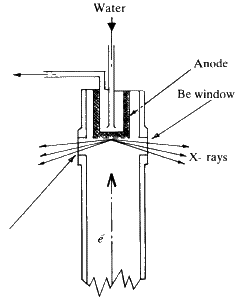
Figure 1 shows schematically a simple X-ray tube. A very high voltage is placed across the electrodes in the two ends of the tube and the tube is evacuated to a low pressure, about 1/1 000 mm of mercury. The current flows between the two electrodes and the electrons carrying this strike the metal target. This causes the emission of X-rays. If one plots a graph of the wavelength of the X-rays emitted against their intensity for varying applied accelerating voltages one obtains results of the kind in Fig. 2. The target for Fig. 2 would be tungsten.
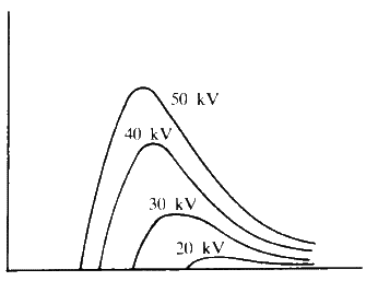
The curves are typical of black body radiation. What is interesting is the very sharp cut-off at short wavelength. This minimum wavelength, lambda minimum, corresponds to the maximum efficiency of conversion of the kinetic energy to electromagnetic radiation; in other words if we use Planck's equation, ![]() , we can calculate lambda minimum. If the accelerating voltage is V, then this minimum is 1.240
, we can calculate lambda minimum. If the accelerating voltage is V, then this minimum is 1.240 ![]() 10-6 m. If we now change the target to a metal of a smaller atomic number such as copper or molybdenum, then we observe very sharp spikes appearing above this smooth background radiation - Fig. 3.
10-6 m. If we now change the target to a metal of a smaller atomic number such as copper or molybdenum, then we observe very sharp spikes appearing above this smooth background radiation - Fig. 3.
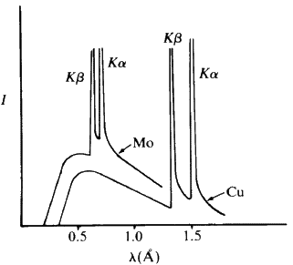
These very sharp spikes are called characteristic lines and the X-radiation is termed characteristic radiation. These sharp lines are caused by electrons being knocked out of the K shell of an atom and then the electrons from the L shell cascading down into the vacancies in this K shell. The energy emitted in this process corresponds to the so-called K alpha and K beta lines. If several metals are present in the target, each will emit its characteristic radiation independently. This property can be used to determine qualitatively which elements are present in an alloy by making it the target in an X-ray tube and then scanning all wavelengths emitted by the target. Typical targets and their related constants are given in Table 1.
| Cr | Fe | Cu | Mo | |
| Z | 24 | 26 | 29 | 42 |
| 2.2896 | 1.9360 | 1.5405 | 0.70926 | |
| 2.2935 | 1.9399 | 1.5443 | 0.71354 | |
| 2.2909 | 1.9373 | 1.5418 | 0.71069 | |
| 2.0848 | 1.7565 | 1.3922 | 0.63225 | |
| V, 0.4mil |
Mn, 0.4mil | Ni, 0.6 mil | Nb, 3mils | |
| Ti | Cr | Co | Y | |
| Resolution, Å | 1.15 | 0.95 | 0.75 | 0.35 |
| Critical potential, kV | 5.99 | 7.11 | 8.98 | 20.0 |
| Operating conditions, kV: | 30-40 | 35-45 | 35-45 | 50-55 |
| half- or full-wave-rectified, mA | 10 | 10 | 20 | 20 |
| constant potential, mA | 7 | 7 | 14 | 14 |
*![]() is the intensity-weighted average of
is the intensity-weighted average of ![]() and
and ![]() and is the figure usually used for the wavelength when the two lines are not resolved.
and is the figure usually used for the wavelength when the two lines are not resolved.
![]() 1 mil =0.001 inch = 0.025 mm.
1 mil =0.001 inch = 0.025 mm.
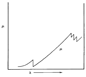
It is fairly obvious that X-rays can be absorbed by solids, and this absorption phenomenon can be described by a very simple equation. The observed intensity I is given by: ![]() where
where ![]() is a linear absorption coefficient and t is the path length through which the X-rays are moving. The value of this absorption coefficient increases as the atomic number of the element concerned increases. Also, if we plot
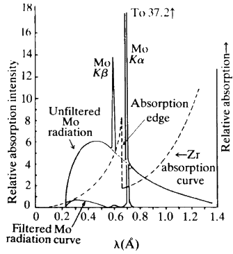
is a linear absorption coefficient and t is the path length through which the X-rays are moving. The value of this absorption coefficient increases as the atomic number of the element concerned increases. Also, if we plot ![]() against wavelength of the X-rays being absorbed for any one given element, we find a rather unusual curve (see Fig. 4). A smooth curve in this plot is followed by very sharp jumps. These discontinuities are called absorption edges and they occur at the wavelength corresponding to the energy needed to knock an electron out of an atomic orbital in the material that is doing the absorbing. In particular, the K absorption edge of an element lies very slightly to the short wavelength side of the K beta lines for that element. Like the characteristic lines, the absorption edge shifts to longer wavelength with decrease in atomic number. If you look now at Fig. 5, you will see that the absorption curve for the element zirconium when superimposed on the X-ray emission curve for the element molybdenum is such that the absorption edge of zirconium comes directly between the K beta and K alpha lines of molybdenum. In other words, if we pass Mo radiation through a sheet of Zr metal, the Zr metal will absorb the beta Mo radiation far more strongly than the alpha radiation. Figure 5 also shows schematically what the resulting distribution of radiation intensities will look like after filtering.
against wavelength of the X-rays being absorbed for any one given element, we find a rather unusual curve (see Fig. 4). A smooth curve in this plot is followed by very sharp jumps. These discontinuities are called absorption edges and they occur at the wavelength corresponding to the energy needed to knock an electron out of an atomic orbital in the material that is doing the absorbing. In particular, the K absorption edge of an element lies very slightly to the short wavelength side of the K beta lines for that element. Like the characteristic lines, the absorption edge shifts to longer wavelength with decrease in atomic number. If you look now at Fig. 5, you will see that the absorption curve for the element zirconium when superimposed on the X-ray emission curve for the element molybdenum is such that the absorption edge of zirconium comes directly between the K beta and K alpha lines of molybdenum. In other words, if we pass Mo radiation through a sheet of Zr metal, the Zr metal will absorb the beta Mo radiation far more strongly than the alpha radiation. Figure 5 also shows schematically what the resulting distribution of radiation intensities will look like after filtering.
In most X-ray work only one well-defined wavelength of radiation is needed and so the X-rays are filtered. Filtering is probably the cheapest and simplest way of obtaining approximately monochromatic X-rays. One can achieve far 'cleaner' radiation by using a so-called monochromator, however, the cost of the monochromator could be 10,000 times the cost of a thin sliver of metal of the correct thickness. Table 2 shows suitable filters for various radiations.
| Target material | Thickness, mm | Thickness, in. | g per cm2 | Per cent loss, |
|
| Ag | Pd | 0.092 | 0.0036 | 0.110 | 74 |
| Rh | 0.092 | 0.0036 | 0.114 | 73 | |
| Mo | Zr | 0.120 | 0.0047 | 0.078 | 71 |
| Cu | Ni | 0.023 | 0.0049 | 0.020 | 60 |
| Ni | Co | 0.020 | 0.0008 | 0.017 | 57 |
| Co | Fe | 0.019 | 0.0007 | 0.015 | 54 |
| Fe | Mn | 0.018 | 0.0007 | 0.013 | 53 |
| Mn2O3 | 0.042 | 0.0017 | 0.019 | 59 | |
| MnO2 | 0.042 | 0.0016 | 0.021 | 61 | |
| Cr | V | 0.017 | 0.0007 | 0.010 | 51 |
| V2O5 | 0.056 | 0.0022 | 0.019 | 64 |
Generally speaking the source of X-rays used will be a commercial generator. Typical X-ray tubes fitted to these generators will have life times of 5000 to l0,000 h, but incorrect handling can reduce the life time very severely. The two most commonly used targets are copper and molybdenum but certain problems may require other wavelengths. For example, if an element two to five places left of copper in the periodic table is being studied, fluorescent radiation is emitted and will completely blacken the film. Cobalt ![]() radiation can be used for samples containing iron without causing fluorescence as would be the case with Cu
radiation can be used for samples containing iron without causing fluorescence as would be the case with Cu ![]() radiation. Of course the emission of this fluorescent radiation is itself an important phenomenon which can be used for analysis as will be described later.
radiation. Of course the emission of this fluorescent radiation is itself an important phenomenon which can be used for analysis as will be described later.
Nowadays X-ray generators are available with highly stabilised power supplies, though of course such apparatus is very expensive. It is necessary when Geiger counters or solid state detectors are being used to measure X-ray intensities, but for photographic work a high degree of stability is not so necessary.
The actual window through which the X-rays emerge is usually made of beryllium--which has an atomic number of only 4 and therefore very low absorption. The windows are delicate and should not be touched.
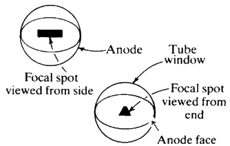
X-ray tubes are sometimes constructed so that two of the windows will provide a line focus while the other two provide what is called a point focus. This is shown diagrammatically in Fig. 6. The line focus is most suitable for powder work but the point focus should always be used for single crystal studies. The tube is clearly marked so there can be no mistaking which of the windows corresponds to either the line or the point focus.
2. Safety and other practical considerations
An X-ray tube operating at about 40,000 V and 25 mA, is converting 1 kW of power, and the X-radiation coming from that tube is extremely dangerous. If you put your hand within 1 or 2 cm of that tube, and allow the full blast of radiation from the window to strike your hand, even for a short time you will get 3rd degree burns and these burns will not heal. The penetrating power of the X-rays, of course, depends very much on the wavelength. Copper K alpha radiation, wavelength about 1.5 ![]() 10-10 m, will penetrate up to 2 m in air and the penetration is still so great at that range, that you can observe it on a zinc sulphide screen. If you use a sensitive Geiger counter, you will find that the radiation can still be detected at a much greater distance. The penetration of molybdenum radiation is even greater.
10-10 m, will penetrate up to 2 m in air and the penetration is still so great at that range, that you can observe it on a zinc sulphide screen. If you use a sensitive Geiger counter, you will find that the radiation can still be detected at a much greater distance. The penetration of molybdenum radiation is even greater.
Anyone planning to work with X-rays at all, should get in contact with the appropriate local safety service. They will give details about what standards should be applied, and where one can get the radiation stickers and brightly coloured emblems to warn passers-by that there are X-rays around. They will also supply film badges which all workers should wear if they are constantly near the X-ray source. In my laboratory, I keep one film badge on the generator constantly rather than wear it on a laboratory coat, because most of the time there is no person standing next to the generator. The idea of keeping the film badge on the generator is to pick up an average background scatter. In our case, the scatter from the Philips generator is very small indeed.
(The only way to get any readable results on the film badge is to deliberately expose the film badge directly to the beam! Under these conditions the film badge is burnt so black that it is not readable on the densitometers at the radiation safety offices. This action will normally result in a frantic telegram asking whether you are still alive!)
Nowadays most generators and cameras are fitted with mechanical and electrical interlocks but regulations differ considerably from one country to another so we shall not go into detail. The importance of good safety practice however cannot be overemphasized.
An X-ray generator contains an extremely large capacitor, so when the generator is switched off, it is still not completely dead, electrically speaking, and in fact very large charges may still be held on the capacitor within the generator for anything up to 15 min. Anyone planning to open up the generator to do any adjustments inside, should never do it immediately the machine is turned off, otherwise there is danger of a 40,000 V shock.
When a generator is started up for the first time after quite a long lay-off, you must remember that you are dealing with very sensitive electronic apparatus and an X-ray tube which will not appreciate a very large thermal or electrical shock. The correct sequence is to switch on the generator but not to apply the high voltage to the tube for 5 min at least. Once the generator has warmed up, then the high voltage may be turned on. The high voltage should be left at the minimum value for 5 or even 10 min and then the voltage and current settings may be slowly increased, usually step by step, to the required values. If you are using the generator every day, this process need not be followed, but if the generator has been shut down for about a month, then the applied voltage should never be increased suddenly, otherwise it is quite possible to detonate the X-ray tube.
The converse applies equally well when the generator is to be switched off. The high voltage and the tube current should be reduced gradually from their maximum operating values down to the minimum values. The high voltage should then be switched off while still leaving the generator electronic circuits and the tube filament switched on. After a further 5 min one can switch off the generator completely. This process allows the target of the tube to cool down because the cooling water is still flowing through the generator even when the high voltage is off. Once you switch off all the power to the generator, the cooling water normally does not flow. If you switch off a generator running at 40,000 V by just punching 'OFF', the applied voltage is removed from the tube, the water flow immediately stops, with the results that the target becomes badly over-heated. This sort of practice will ruin a tube very quickly.
It is important to remember that probably more trouble is caused by a poor supply of cooling water than by anything else. Generators are sensitive not only to the volume flowing through them, but also to the pressure of the water. (A generator will not start unless there is an adequate flow of water at the correct pressure.) It is, therefore, very necessary to maintain a constant flow at an adequate pressure. The best way to do this is to have a closed circuit water supply with a small pump sending the water through the generator and then back to the ballast tank. Normally some kind of a cooling device is also needed; (a small water tower is suitable) and then this will maintain the temperature of the water. There are safety devices built into every generator and these devices fairly obviously will be sensitive to dirt in the water and so it is necessary to put at least one and perhaps two filters (one coarse, one fine) into the water line. With such an arrangement, one can operate continually for 4 or 5 years with the same 100 gal of water running through the generator. The alternative is to try to use tapwater from the mains and simply pour this water through the generator at the rate of 1,000 gal/day straight down the drain. This may sound cheap and easy but it is not, because there is no guarantee whatsoever that the water in the main will be coming through at 70 lb/in2 constantly day and night. If you want to operate your generator day and night this is what you need. In practice, the mains pressure can fluctuate between 20 and 100 lb/in2. A perfectly adequate water pump and cooling system can be installed quite cheaply if you are prepared to build some of it yourself. Unfortunately, the smallest commercially available cooling towers are far too big for this particular job. A half horsepower motor and a small Mono pump are perfectly adequate to supply water at 70 lb/in2, enough to cool about 3 kW of power. In our laboratory we cool 3 generators from one small pump.
3. Structure of crystals
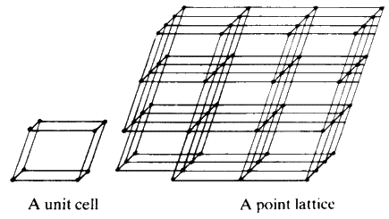
Large crystals are characterized by having well-defined smooth faces and the angle between any pair of these faces for any one type of crystal is always fixed. In addition, it is possible to cleave certain crystals in well-defined directions. A large crystal of sodium chloride (table salt) may be cleaved many many times, gradually reducing it in size, and every time it is cleaved one still obtains crystals that are physically similar in appearance. This phenomenon is what led Hauy to suggest that a crystal is built up of an infinite number of tiny unit cells, which are stacked together in a 3-dimensional lattice by simple translation. A high proportion of all solid matter is built in this way on an atomic scale, even though the material may not show outward signs of crystallinity.Each of the unit cells (Fig. 7) is identical to all others and the symmetry and shape of the whole crystal depends on the symmetry of that cell.
In general, materials can be divided into various classes according to the bonding holding the solid together. Metals constitute one well-known class. Typical organic compounds, such as naphthalene, crystallize into what are called molecular or van der Waals solids. These are characterized by very low melting points because the melting point is a function of the weak attractions between the organic molecules. Very hard materials like quartz and diamond are typical of crystals which are held together by a 3-dimensional network of very strong covalent bonds. Sodium chloride is a typical example of an ionic solid.
The ideas of the unit-cell, the lattice and the symmetry of crystals are abstractions which can be discussed without reference to specific crystals. But in order to come to a real understanding of the subject it is important to gain first hand experience of how the abstractions operate in real materials by a careful study of crystal models.
What is said about the symmetry of the unit cells or about the symmetry of the faces of the crystals, or any other comment that is made about the lattices or the Miller indices, applies equally well to all possible classes of crystalline material. It does not matter which we are dealing with.
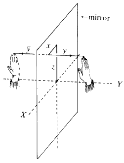
First and foremost in importance is the idea of symmetry. Does the molecule that we are going to deal with have certain symmetry properties? Does the crystal that we are going to look at have certain symmetry properties? Probably the best place to start with symmetry is your left hand; it has symmetry 1: it cannot be converted into itself by any rotation or movement. Similarly, your right hand has symmetry 1: it cannot be transformed into itself by any motion. However, if you place the two hands together so the palms are up and the little fingers are touching edge to edge, then down the line where the two hands join there is a mirror plane. In other words, if the left hand is removed and a mirror is placed next to the right hand, the reflection in the mirror is to all intents and purposes exactly the same as the left hand so these two hands stuck together have the symmetry m, meaning mirror symmetry. If you place the two hands palm to palm, the same thing applies (see Fig. 8). There is a mirror plane of symmetry where the two palms touch; so if you remove the right hand and place a mirror there and look into it, the left hand appears on the right hand side behind the mirror and it looks just the way the right hand did. If you put the two hands back together, right where the two palms touch is a mirror plane of symmetry.
Now make the two thumbs touch at their tips and look at the backs of the hands. Again there is a mirror plane between the hands. Now rotate one hand about the point of contact of the thumbs so that the fingers of each hand point in opposite directions. The back of one hand and the palm of the other are now visible.
The two hands are now related by what is called a centre of inversion at the point of contact of the thumb. The hands can be separated and, if maintained in the same relative orientation there will still be a centre of inversion between them (Fig. 9).
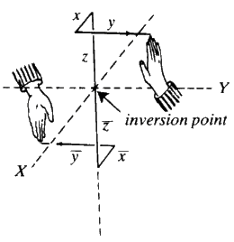
Mathematically speaking, if the coordinates of any point on one hand, relative to the centre of inversion, are x, y and z, then the coordinates of the corresponding point on the other hand will be -x, -y and -z.
To a first approximation, a person has a mirror plane of symmetry splitting him in half right down the middle of the face and the body. If two people link arms with bent elbows so that one faces forward and the other faces back then that pair (as long as they are both male or both female) has approximately a two-fold axis running parallel to the line of their bodies, perpendicular to the floor, through the point where the two elbows meet. If they turn around 180![]() , they are (for all intents and purposes) the same as they were when they started. They would represent a molecule which has a two-fold axis of symmetry.
, they are (for all intents and purposes) the same as they were when they started. They would represent a molecule which has a two-fold axis of symmetry.
Probably the best way to get a feeling for symmetry elements in molecules and in crystals, is to draw a few yourself, look at a fair number of illustrations in the reference text books and, as mentioned earlier, study crystal models.
4. Classification of crystals
The abstractions of unit cells, lattice and symmetry to which reference has already been made lead to the possibility of classifying all crystals into well defined systems. On mathematical grounds it can be shown that there are only 7 possible unit-cell types (the 7 crystal systems) but, because some are capable of replicating themselves in a lattice in more than one way there are 14 possible lattices (the so-called Bravais lattices (Table 3)).
| System | Axial lengths and angles | Bravais lattice | Lattice symbol |
| Cubic | Three equal axes at right angles |
Simple | P |
| Body-centered | I | ||
| Face-centered | F | ||
| Tetragonal | Three axes at right angles, two equal |
Simple | P |
| Body-centered | I | ||
| Orthorhombic | Three unequal axes at right angles |
Simple | P |
| Body-centered | I | ||
| Base-centered | C | ||
| Face-centered | F | ||
| Rhombohedral* | Three equal axes, equally inclined |
Simple | R |
| Hexagonal | Two equal coplanar axes at 120 third axis at right angles |
Simple | P |
| Monoclinic | Three unequal axes, one pair not at right angles |
Simple | P |
| Base-centered | C | ||
| Triclinic | Three unequal axes, unequally inclined and none at right angles |
Simple | P |
* Also called trigonal.
There are 32 ways in which symmetry elements that can be detected by visual or morphological examination can be arranged (the 32 point groups) but, if all the symmetries possible on an atomic scale are included there are 230 possible arrangements (the 230 space groups).
It is interesting and important to remember that no crystal can have a 5-fold axis of symmetry. However, individual molecules can have such an axis of symmetry. A crystal cannot have a 5-fold axis because there is no way of packing by translation an infinite number of unit cells which have a pentagonal cross section so that they completely fill space.
Because space group symmetry is of little importance in the applications to be described, it will not be dealt with. Of course, a full understanding of the 230 space groups is necessary for anyone undertaking the determination of molecular structure by X-ray diffraction.
It will now be useful to consider the concept of families of planes running through a crystal and their labelling by the use of Miller indices. We will start by considering lines in two dimensions.
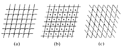
If we join the corners of the unit cells, or any other point in the cell, by straight lines we generate families of lines. All the lines in a family are parallel to each other and run through the same number of lattice points. Figure 10 shows three examples.
Consider Fig. 11(a). Through each cell there is only one plane. Start from the lattice point at the bottom left hand corner, and consider that as the origin. You will travel along the vertical direction one cell edge before you encounter such a line; if you travel along the horizontal axis you will move one cell edge before you encounter a line. Consider the set of planes in sketch b. Start at the origin and move along the vertical axis. You will come in contact with three lines before you reach the first lattice point along that edge. If you move along the horizontal direction you will come in contact with only one line before you reach the first lattice point. In sketch c in moving along the vertical direction from the origin, to the first lattice point, you contact only one line; moving along the horizontal direction, you cross two lines. It should be fairly obvious that you can describe the geometry of these lines simply in terms of how many cut one unit cell edge or into what number of equal size pieces this family of lines will cut one unit cell edge. In sketch a, the family cuts the vertical axis into one and the horizontal axis into one. In sketch b, the vertical axis is cut into three, the horizontal axis, one. In sketch c, the vertical axis is cut once while the horizontal is cut twice. So the planes in sketch a could be labelled 1:1; those in b could be labelled 3:1, those in c could be labelled 1:2. The sign of the slope of the planes is obviously different between b and c and so we will have to define the positive and negative directions along the edges of the cell. Define the vertical direction, starting from the bottom left hand corner, going up as positive and horizontal, starting at the left hand corner, going across to the right as positive. We would then find that in a, you could number these planes as (+1 +1), in b they would be labelled (+3 +1) and in c the label would be (+1 -2). These numbers that can be assigned to the lines are called Miller Indices, and they are characteristic of these lines. It is obvious that the larger the Miller Indices that we can assign to the family of lines, the closer together these lines will be; in other words, the smaller will be the perpendicular distance between adjacent parallel lines. It should also be obvious that the distance between any pair of lines will be the same no matter where you are in the crystal because all the unit cells are the same size. What was done here in two dimensions is easily extended to three dimensions. Thus, any plane running through a crystal and passing through the set of lattice points--in other words through the corners of the unit cells--can be identified by a triplet of integers; the Miller Indices. The symbols used are the alphabetical letters (hkl). We can describe any plane in a crystal by three integers and these numbers can have + or - signs. A negative index, -n, is usually written as ![]() for convenience. Typical families of widely spaced planes might be: (110),
for convenience. Typical families of widely spaced planes might be: (110), ![]() etc.: planes such as (742),
etc.: planes such as (742), ![]() etc., would be much closer together.
etc., would be much closer together.
5. Diffraction of X-rays
We will examine in turn what happens when X-rays strike a single atom, when a plane wave front of X-rays strikes a line of atoms, when a beam of X-rays strikes a two-dimensional net of atoms and finally a 3-dimensional lattice of atoms.
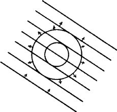
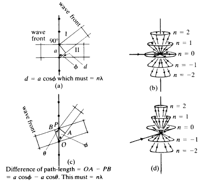
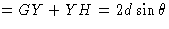
When a wavefront of X-rays strikes an atom, the electrons in that atom interact with the X-rays and immediately re-emit the X-radiation, normally without change of wavelength, and the X-radiation that is emitted by the atom is emitted as a spherical wavefront (Fig. 12). This, of course, is an ideal situation which we cannot observe in practice. Consider a line of identical atoms, distance a apart. Let a beam of wavelength ![]() strike this line of atoms at an angle
strike this line of atoms at an angle ![]() . Each of these atoms immediately begins to emit radiation in the form of spherical wavefronts (Fig. 13). If one observes the scattered radiation in the plane of the incident beam and scans all possible angles, the requirement for seeing a beam of enhanced intensity is that the path-length difference between the advancing incident wavefront and the advancing diffracted wavefront shall be a whole number of wavelengths.
. Each of these atoms immediately begins to emit radiation in the form of spherical wavefronts (Fig. 13). If one observes the scattered radiation in the plane of the incident beam and scans all possible angles, the requirement for seeing a beam of enhanced intensity is that the path-length difference between the advancing incident wavefront and the advancing diffracted wavefront shall be a whole number of wavelengths.
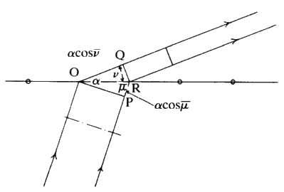
Consider Fig. 14. The length PR-OQ should be equal to n![]() wavelength
wavelength ![]() . If that situation holds, then the observer looking along the lines of the arrows will see that the scattered radiation is very intense at that angle: there is constructive interference. If the observer moves away from that particular angle there will be no enhanced scattered radiation. It is important to notice that, while the sketch is two-dimensional, each atom is giving off a spherical wave of radiation. The directions of scattering thus constitute the surface of a series of cones (see Fig. 15). The largest cone angle corresponds to a difference of one wavelength between the incident and the diffracted radiation. The angle of deviation increases and the cone angle decreases as the integer becomes 1, 2, 3 and so on. It is fairly obvious that for cosine
. If that situation holds, then the observer looking along the lines of the arrows will see that the scattered radiation is very intense at that angle: there is constructive interference. If the observer moves away from that particular angle there will be no enhanced scattered radiation. It is important to notice that, while the sketch is two-dimensional, each atom is giving off a spherical wave of radiation. The directions of scattering thus constitute the surface of a series of cones (see Fig. 15). The largest cone angle corresponds to a difference of one wavelength between the incident and the diffracted radiation. The angle of deviation increases and the cone angle decreases as the integer becomes 1, 2, 3 and so on. It is fairly obvious that for cosine ![]() and it is this condition which tells you the maximum number of cones that will be observable from a line of atoms of spacing d for radiation of wavelength
and it is this condition which tells you the maximum number of cones that will be observable from a line of atoms of spacing d for radiation of wavelength ![]() . Consider now a second line of atoms at some angle to the first line: a two-dimensional net. Consider the second line of atoms quite independently from the first line and it is fairly obvious that the second line of atoms when irradiated by the X-rays will generate a series of cones also obeying the same criteria. Thus the two-dimensional net will behave as if it were simply two lines of atoms and produce two families of intersecting cones. It should be fairly obvious that for two sets of cones with a common origin but with their axes non-collinear, the intersection of these cones will consist of a series of lines. Thus, for a two-dimensional net, very strong constructive interference will be seen only along certain well defined directions in space, and no longer anywhere along the surface of the cone as was observed for one line of atoms (see Fig. 16).
. Consider now a second line of atoms at some angle to the first line: a two-dimensional net. Consider the second line of atoms quite independently from the first line and it is fairly obvious that the second line of atoms when irradiated by the X-rays will generate a series of cones also obeying the same criteria. Thus the two-dimensional net will behave as if it were simply two lines of atoms and produce two families of intersecting cones. It should be fairly obvious that for two sets of cones with a common origin but with their axes non-collinear, the intersection of these cones will consist of a series of lines. Thus, for a two-dimensional net, very strong constructive interference will be seen only along certain well defined directions in space, and no longer anywhere along the surface of the cone as was observed for one line of atoms (see Fig. 16).
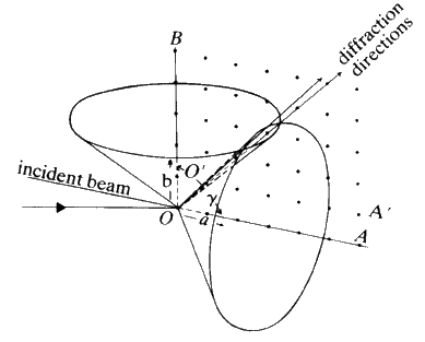
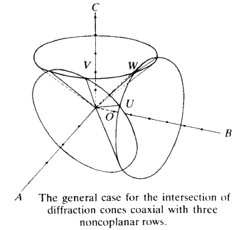
To extend this idea into three dimensions you need only add another line of atoms non-coplanar with the first net. Irradiate this line of atoms with the X-ray beam and, as before, a series of cones is formed. This family can only have a line of intersection common with those of the first two under the special condition that UV and W are coincident (see Fig. 17). The result is that, for a three dimensional lattice of atoms irradiated by X-radiation, strong constructive interference will only occur in specific directions and for specific conditions of incidence. In other words one will not observe constructive interference unless one stands exactly in the right place in space. This type of construction was done by Laue about 1912. Although it is mathematically very straightforward, it is very difficult to picture in three-dimensions what is going on. Fortunately for us, Bragg in 1913 saw that the conditions for constructive interference of X-rays were equivalent to that of a simple plane reflecting the X-ray radiation with the condition that the plane could be described by a triplet of Miller indices. We can take any plane (hkl) in our crystal and we will now consider not spacings between atoms or lattice points, but spacings between the planes.
 , which must
Consider Fig. 18. The incident X-radiation strikes the planes (hkl) at an angle ![]() . The spacing between these planes is d. We will assume that the X-rays are reflected in exactly the same way as light will be reflected from a mirror so that the reflected beam leaves the plane at angle
. The spacing between these planes is d. We will assume that the X-rays are reflected in exactly the same way as light will be reflected from a mirror so that the reflected beam leaves the plane at angle ![]() . The requirement for constructive interference is very simple. Once again it is that the path length difference between the incoming and the outgoing beams should be a whole number of wavelengths. It is very easy to show that the path difference is equal to
. The requirement for constructive interference is very simple. Once again it is that the path length difference between the incoming and the outgoing beams should be a whole number of wavelengths. It is very easy to show that the path difference is equal to ![]() and the final result is
and the final result is ![]() . This is called Bragg's law, and it is of considerable importance in X-ray crystallography. The maximum value that
. This is called Bragg's law, and it is of considerable importance in X-ray crystallography. The maximum value that ![]() will ever have is 1. For
will ever have is 1. For ![]() and the X-ray strikes perpendicular to the face of the crystal and is reflected back along the incident path. For this case,
and the X-ray strikes perpendicular to the face of the crystal and is reflected back along the incident path. For this case, ![]() ; the minimum d-spacing that we can ever observe with X-rays in any crystal will be equal to one half of the incident wavelength of the X-rays. What is interesting here, is that Bragg included the numerical value n (the integer) because he chose planes whose Miller indices (hkl) were prime numbers. In other words, Bragg's planes would be called (111) but never (222) or (333). This followed the normal conventions used in geology. He would talk about the plane (111) and then he would consider the n in the equation to be the 1st, 2nd, 3rd, 4th and so on order of reflection from that plane. For the single crystal X-ray crystallographer the numerical value of n is normally said to be equal to 1 and then we would simply use the equation
; the minimum d-spacing that we can ever observe with X-rays in any crystal will be equal to one half of the incident wavelength of the X-rays. What is interesting here, is that Bragg included the numerical value n (the integer) because he chose planes whose Miller indices (hkl) were prime numbers. In other words, Bragg's planes would be called (111) but never (222) or (333). This followed the normal conventions used in geology. He would talk about the plane (111) and then he would consider the n in the equation to be the 1st, 2nd, 3rd, 4th and so on order of reflection from that plane. For the single crystal X-ray crystallographer the numerical value of n is normally said to be equal to 1 and then we would simply use the equation ![]() but the d in the equation would be for a plane whose Miller indices can be either prime numbers or non-prime. Notice something else about the Bragg equation. Theta is a variable, in other words it is an angle which you can choose simply by rotating the crystal relative to the X-ray beam. The wavelength has a fixed value and d is obviously a fixed value determined by the size of the unit cell and the Miller indices. If we write down the equation as
but the d in the equation would be for a plane whose Miller indices can be either prime numbers or non-prime. Notice something else about the Bragg equation. Theta is a variable, in other words it is an angle which you can choose simply by rotating the crystal relative to the X-ray beam. The wavelength has a fixed value and d is obviously a fixed value determined by the size of the unit cell and the Miller indices. If we write down the equation as ![]() and fix
and fix ![]() in our experiment, we see that the experimentally observed value of
in our experiment, we see that the experimentally observed value of ![]() is a direct measure not of the d spacing but of the reciprocal of the d spacing of the planes. Notice also that somehow or other we are looking at perpendiculars to these planes because this d spacing is the perpendicular distance between planes of the crystal. For this reason, Ewald (1912) constructed what he called a reciprocal lattice. A reciprocal lattice is merely a construction that consists of normals drawn to all possible lattice planes whose indices are (hkl). These normals radiate from a common origin (the point 0, 0, 0 in the unit cell) and each normal terminates at a distance from the origin, proportional to the reciprocal of the d-spacing of the plane (hkl). Consider Fig. 19. What is interesting about it, is that each family of planes whose Miller indices are (hkl) is described by only one point in the reciprocal lattice: you may have an infinite number of planes of indices (hkl) but they correspond to one point (hkl) in the reciprocal lattice. The geometrical relationship between real lattices and unit cells and these reciprocal lattices and reciprocal cells are fairly complex. They will not help us directly with the applications that we want to consider in this article, therefore it is best that we stop the discussion of reciprocal lattices at this point and proceed to some other aspects of X-rays and interactions of X-radiation with crystals.
is a direct measure not of the d spacing but of the reciprocal of the d spacing of the planes. Notice also that somehow or other we are looking at perpendiculars to these planes because this d spacing is the perpendicular distance between planes of the crystal. For this reason, Ewald (1912) constructed what he called a reciprocal lattice. A reciprocal lattice is merely a construction that consists of normals drawn to all possible lattice planes whose indices are (hkl). These normals radiate from a common origin (the point 0, 0, 0 in the unit cell) and each normal terminates at a distance from the origin, proportional to the reciprocal of the d-spacing of the plane (hkl). Consider Fig. 19. What is interesting about it, is that each family of planes whose Miller indices are (hkl) is described by only one point in the reciprocal lattice: you may have an infinite number of planes of indices (hkl) but they correspond to one point (hkl) in the reciprocal lattice. The geometrical relationship between real lattices and unit cells and these reciprocal lattices and reciprocal cells are fairly complex. They will not help us directly with the applications that we want to consider in this article, therefore it is best that we stop the discussion of reciprocal lattices at this point and proceed to some other aspects of X-rays and interactions of X-radiation with crystals.
 |
We accept at this stage that any set of planes in a crystal will cause a reflection of the X-ray beam if the set of planes is set at the right angle to the incident X-ray beam. The question now is how strongly will this set of planes reflect the X-rays? Will they necessarily reflect the incoming beam strongly or will they reflect it fairly weakly? The intensity of the reflected beam will be proportional to the product of the intensity of the incident beam and the concentration or density of electrons in the plane that is reflecting the beam. Note: It is the concentration of electrons , not of atoms, because it is the electrons surrounding the atoms that cause the scattering of the X-rays. It should be obvious that, if we know the size of the unit cell and if we know exactly where all the atoms are in that unit cell and if we know the atomic number of each of these atoms (in other words if we know how many electrons are associated with each atom in that cell), we should be able to calculate for any chosen plane with Miller indices (hkl) exactly what the concentration of electrons in that plane will be. In other words, if we know the structure of the unit cell, we should be able to calculate the intensity with which any chosen plane in that cell will scatter X-rays. In fact, this is very easy to do and the name given to such a calculated value is the Structure Factor.
Consider the reverse situation. Imagine that we know the size of the unit cell and that we can measure the intensities of reflection from all possible planes. It appears that from this information we should be able to calculate the positions of the atoms in the cell and not only that, but also the relative number of electrons per atom. The problem of working out where the atoms are in the unit cell from the observed d-spacings and intensities of reflection is called 'solving a crystal structure'. This is one thing we will not attempt to do in this course, because what may sound very easy is, in fact, extremely complicated under some circumstances. All that is important at this stage, is to bear in mind that the intensity with which any family of planes can reflect an X-ray beam is directly proportional to the concentration of electrons in those planes. It is obvious that all compounds whose formulae are different, or whose unit cells are different, must have a different collection of possible d-spacings and of different intensities of reflection. The combination of different d-spacings and different intensities is characteristic of any crystalline material and we can use the observed pattern of spacings and intensities of the reflections as a way of identifying an unknown compound in a specific crystalline phase. It will be as characteristic of a particular crystal structure as a fingerprint is of a specific person.
6. Laue, powder and single-crystal methods
The Laue method
Laue in his very first experiments used white radiation of all possible wavelengths and allowed this radiation to fall on a stationary crystal. The crystal diffracted the X-ray beam and produced a very beautiful pattern of spots which conformed exactly with the internal symmetry of the crystal. Let us analyse the experiment with the aid of the Bragg equation. The crystal was fixed in position relative to the X-ray beam, thus not only was the value for d fixed, but the value of ![]() was also fixed (see Fig. 20).
was also fixed (see Fig. 20).
The only possible variables therefore are the integer n and wavelength ![]() , with the result that in the Laue photograph each observed reflection corresponds to the first order of reflection of a certain wavelength, the second order of half the wavelength and a third order of a third of the wavelength, and so on. The Laue photograph which is obtained from a single crystal is simply a stereographic projection of the planes of the crystal.
, with the result that in the Laue photograph each observed reflection corresponds to the first order of reflection of a certain wavelength, the second order of half the wavelength and a third order of a third of the wavelength, and so on. The Laue photograph which is obtained from a single crystal is simply a stereographic projection of the planes of the crystal.
The powder method
Now try a different experimental arrangement. Rather than using white radiation, take monochromatic X-radiation of one fixed wavelength and place the crystal in front of the beam. If one plane is set at exactly the correct value of
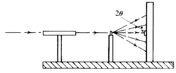
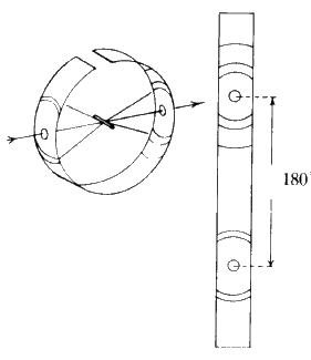
The powder camera (Fig. 21) consists of a metal cylinder at the centre of which is the sample. The powdered material is often glued onto a glass rod with clear fingernail varnish. A strip of X-ray film is placed inside the cylinder. Punched into one side of the film is a hole for the beam collimator and punched into the other side 180![]() away, is another hole through which a beam catcher can be placed. The camera is closed by a light-tight lid and placed in front of the X-ray beam. The pattern on the film is shown on the right of Fig. 22.
away, is another hole through which a beam catcher can be placed. The camera is closed by a light-tight lid and placed in front of the X-ray beam. The pattern on the film is shown on the right of Fig. 22.
This technique can be adapted to photographing wires and sheets of metal. A flat film is also commonly used for recording reflections at small ![]() angles.
angles.
Moving crystal and moving film methods
The rotation method
The Laue method dealt with white radiation, a stationary single crystal and a fixed sheet of film. The rotation method deals with monochromatic radiation, a moving single crystal and a fixed sheet of film.
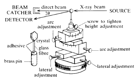
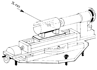
A single crystal (edge lengths between 0.1 and 2 mm) is attached to a glass fibre which is in turn mounted on a spindle. The crystal orientation is adjusted until the crystal can be rotated about a real crystallographic axis (see Fig. 23).
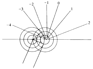
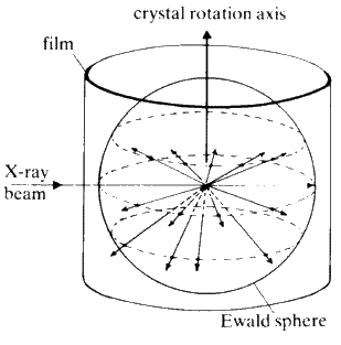
A collimated beam of monochromatic X-rays falls on the crystal perpendicular to the rotation axis, and the crystal is rotated. The various planes in the crystal will reflect the beam as the rotation brings each in turn into the diffracting position, i.e. the Bragg equation is satisfied. Let the rotation axis correspond with the real c axis. All planes (hkl) with a common l index will produce reflections along the surface of a common cone the apex angle of which is defined by the Laue condition ![]() . The film is usually wrapped around the crystal in the form of a cylinder, coaxial with the rotation axis of the camera (see Fig. 24).
. The film is usually wrapped around the crystal in the form of a cylinder, coaxial with the rotation axis of the camera (see Fig. 24).
The photograph obtained consists of individual reflections from the crystal forming straight lines across the film. From the spacing between the lines, the length of the 'rotation' axis of the crystal can be calculated. The symmetry of the pattern of spots on the film gives information about the symmetry of the unit cell.
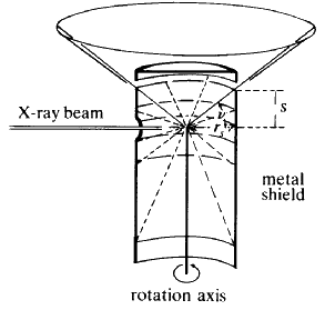
The Weissenberg method
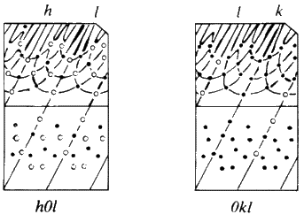
The Weissenberg technique is a development of the rotation technique. A typical camera is shown diagrammatically in Fig. 25. A slotted cylindrical screen is placed between the crystal and the film so that only one cone of reflections can strike the film (see Fig. 26) and then as the crystal is rotated, the film holder is translated parallel to the rotation axis. This results in the reflections (which formed a straight line on the rotation photograph) being spread across the film in a specific 2-dimensional pattern. The screen is movable, so each cone or 'layer' of reflections (n = 0, 1, 2 etc.) can be photographed separately. From these photographs can be calculated the lengths of the other crystallographic axes and the interaxial angles. In addition, the symmetry and space group of the unit cell can be deduced from an analysis of the Miller indices of the reflections which are systematically absent (see Fig. 27).
This is the most common single crystal X-ray camera, and it has been used for the past 40 years for the collection of intensity data for crystal structure elucidation.
The precession method
The precession camera was invented by Buerger in about 1940. This technique uses a flat film holder linked to the crystal oscillation axis. With the instrument set at zero, the X-ray beam must strike the crystal parallel to a real axis and perpendicular to the film. The crystal (and film) is tilted by an angle ![]() of up to 30
of up to 30![]() , and allowed to 'precess' so that the real crystallographic axis traces a cone about the X-ray beam. See Fig. 28.
, and allowed to 'precess' so that the real crystallographic axis traces a cone about the X-ray beam. See Fig. 28.
The motion is complex but results in a photograph that gives an undistorted picture of the 'reciprocal lattice'.
This is the second most common single crystal camera in current use. It is very popular for studies of crystalline proteins.
The reciprocal lattice explorer
The most recent advance in single crystal cameras is the Explorer, invented by Wolfel. This instrument is a combination of a Precession camera and a de Jong camera. This combination produces a complete and undistorted survey of the reciprocal lattice. (The de Jong method records the same reflections as does the Weissenberg method, but with a different instrument geometry that produces a distortion-free result.)
Diffractometers
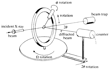
All of the methods described so far use X-ray film for recording the reflections. They may all be modified so that a Geiger counter or other electronic detector can be used to detect both the presence and intensity of each of the reflections. There are now computer-controlled diffractometers available commercially that require only that the crystal be aligned in the X-ray beam and then the instrument will in turn, measure and refine the unit cell dimensions, record all reflections out to a chosen maximum theta-angle, and punch out the values of hkl, intensity, and estimated error for each reflection. The geometry of a 4-circle instrument is shown schematically in Fig. 29.
An automatic diffractometer can easily measure reflections from a single crystal at the rate of one per minute, so the data for any normal crystal structure can be collected in a few days. With the aid of a competent crystallographer and a modern computer, the detailed molecular structure of any molecule of up to 100 atoms (not counting hydrogens) can be solved in less than three weeks. (Compare this with the months or years required by degradative chemical techniques.) All that is needed is: a good crystal, about 0.3 mm cubed, of a derivative containing one atom of atomic number round about 30. For compounds of up to 20 C, N, O, one Cl is adequate; up to 50 C, N, O, one Br is adequate (e.g. a parabromobenzoate is a very useful derivative); for about 100 C, N, O, one Iodine is acceptable, but two Br are probably better. Potassium or rubidium salts are suitable for organic acids.
7. Application to the analysis of materials
There are three distinct properties of X-rays that can be used practically:
- (i)
- Absorption
- (ii)
- Fluorescence
- (iii)
- Diffraction
(i) Absorption
The high penetration by X-rays through material and the variation of absorption by the material with change in thickness naturally leads to the well-known technique of radiography, both medical and industrial. Castings and welds are routinely 'X-rayed' to check for blow-holes or cracks. Because the results are recorded photographically, good reviews of the technique are available from the manufacturers of X-ray film, e.g. Kodak, Ilford, Gevaert.
This technique can also be used to continuously monitor the thickness of rolled sheet and foils and also of plating on sheet metal. All that is required is a source of X-rays on one side of the moving sheet and a Geiger tube on the other. Any variation in thickness will immediately register as a variation in count-rate. The signal could be used via a relay to automatically correct the fluctuation without intervention by any person.
Radiography is in everyday use in many industries. It is used for examining steel-banded tyres, for testing welds, for checking heating elements and for many other purposes: the possibilities are almost limitless.
(ii) Fluorescence
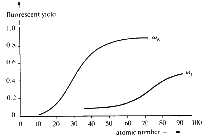
When suitably excited, atoms of every element will emit characteristic radiation whose wavelength is a function of the reciprocal of the square of the atomic number Z of the element. In principle, it is possible to identify the elements in a sample by exciting it and measuring the wavelengths of the characteristic X-rays that are emitted. The efficiency of emission--The Fluorescent Yield--is dependent on atomic number; high with high atomic number and rapidly dropping off as Z drops below about 20 (see Fig. 30).
Increasing the concentration of any element in the sample will result in a proportional increase in the intensity of the fluorescent radiation characteristic of that element. Thus, X-ray fluorescence is simultaneously a qualitative and quantitative technique: ideal for non-destructive analysis of alloys.
In practice the sample is excited by a high intensity beam of X-rays, sometimes monochromatic, sometimes white (or continuous). Not only is the choice of tube target dictated by the type of analysis being done, the correct choice of tube current and potential is just as important.
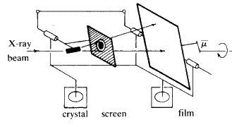
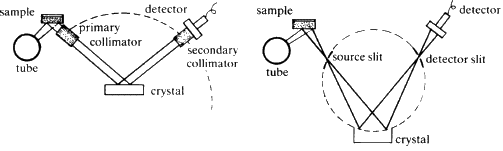
Two typical arrangements for an X-ray spectrometer are shown diagrammatically in Fig. 31. The heart of the instrument is the crystal analyser. It is chosen so that one set of planes of exactly known d-spacing is presented to the fluorescent X-ray beam. The crystal can be rotated so that ![]() can be varied, and then the Bragg equation
can be varied, and then the Bragg equation ![]() , is applied, d is fixed,
, is applied, d is fixed, ![]() can be measured directly hence the wavelength
can be measured directly hence the wavelength ![]() of the diffracted X-ray beam can be calculated. The choice of the analysing crystal is determined by the range of wavelengths which are to be measured, the length of acceptable counting times, and by the type of detector that is to be used.
of the diffracted X-ray beam can be calculated. The choice of the analysing crystal is determined by the range of wavelengths which are to be measured, the length of acceptable counting times, and by the type of detector that is to be used.
There are at least four well-defined types of counters available commercially.
- 1.
- Geiger-Muller
- 2.
- Proportional
- 3.
- Gas flow
- 4.
- Scintillation
The choice of counter is determined by the wavelengths of the X-rays to be detected, required counting rates, sensitivity and acceptable background noise.
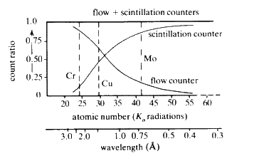
The combination of flow, proportional and scintillation counter has obvious advantages if a wide range of elements are to be analysed (Fig. 32).
 |
| Geiger | Proportional | Gas Flow | Scintillation | |
| Window | Mica | Mica | Mylar/Al | Be/Al |
| Thickness | 3 mg/cm2 | 2.5 mg/cm2 | 6 |
0.2 mm |
| Position | Radial | Axial | Axial | Radial |
| Filling | Ar/Br | Xe/CH4 | Ar/CH4 | -- |
| Pre-amplifier | unnecessary | |||
| Auto-amplification | 109 | 106 | 106 | 106 |
| Useful range (Å) | 0.5-4 | 0.5-4 | 0.7-10* | 0.1-3 |
| Dead time (Micro seconds) | 200 | 0.5 | 0.5 | 0.2 |
| Max. useful count rate | 2 |
5 |
5 |
106 |
| Cosmic background (c/s) | 0.8 | 0.4 | 0.2 | 10 |
| Resolution % (Fe |
-- | 14 | 15 | |
| Quantum counting efficiency | reasonably independent of |
(iii) Diffraction
By far the most important industrial use of diffraction is through the powder technique. Typically this can be used for:
Qualitative analysis
The powder pattern of a sample is recorded, the d spacings (or ![]() angles) and relative intensities of the 10 strongest lines are measured and these are compared with the patterns of known compounds. Many thousand patterns have been recorded and published in the ASTM (JCPDS) Powder Diffraction File and these are available in subdivisions: Minerals, Inorganic, Organic. With experience, it is possible to identify the components in mixtures of up to three compounds.
angles) and relative intensities of the 10 strongest lines are measured and these are compared with the patterns of known compounds. Many thousand patterns have been recorded and published in the ASTM (JCPDS) Powder Diffraction File and these are available in subdivisions: Minerals, Inorganic, Organic. With experience, it is possible to identify the components in mixtures of up to three compounds.
Quantitative analysis
The relative concentration of each of the components in a two-component mixture can be obtained by measuring the relative intensities of two strong non-overlapping lines, one belonging to component A, the other to component B, in the powder pattern of the mixture. A well-known example is the determination of anatase in rutile (see Jenkins and de Vries, 1967).
Structure of alloys
When the components of an alloy are uniformly distributed throughout the metal, the sample will produce a typical powder photograph. If the metal is 'worked' or, in certain cases, cooled, one of the components often 'precipitates'. This can be observed on the powder photograph as 'spots' where previously there were uniform lines. If the atoms of the alloy 'order' (e.g. in ![]() -brass) new lines are formed on the powder film - a 'super-lattice' is said to be formed. These phenomena are easily observed by photographic X-ray techniques.
-brass) new lines are formed on the powder film - a 'super-lattice' is said to be formed. These phenomena are easily observed by photographic X-ray techniques.
Stress determination in metals
If a piece of metal is strained, the unit cell dimensions will be altered slightly. Because the magnitude of the cone angle of a diffraction cone is a function of the d-spacing, any small change in the d-spacing can be observed as a corresponding change in the ![]() angle of the diffracted cone. Thus, accurate measurement of stress can be obtained by measuring the differences in
angle of the diffracted cone. Thus, accurate measurement of stress can be obtained by measuring the differences in ![]() angles from powder (pin-hole) photographs of the specimen made before and after straining.
angles from powder (pin-hole) photographs of the specimen made before and after straining.
Determination of particle size
The angular spread of the reflection from a crystal plane is affected not only by the perfection of the crystal but also by the size of the crystal. As the average size of the crystallites decreases, so the angular spread of the reflection from a powder will increase. After suitable calibration, the half height width of a reflection in a powder diffractogram can be used as quantitative measure of the mean particle size of the sample.
Identification and raw material evaluation
For complex materials (e.g. cement powder, sands, clays), the powder pattern will be correspondingly complex, however, it will be characteristic of the material. Although the pattern cannot be analysed for each of the individual components, similar materials will always exhibit similar patterns. The possible usefulness of different clays as raw materials for cement or brick manufacture can often be quickly determined by comparison of their diffraction patterns with that of an acceptable clay.
Further reading
Azaroff and Buerger, The Powder Method, McGraw-Hill, 1958.
Barrett and Massalski, Structure of Metals, McGraw-Hill, 1966.
Buerger, Crystal Structure Analysis, Wiley, 1960.
Buerger, X-Ray Crystallography, Wiley, 1942.
Cullity, Elements of X-Ray Diffraction, Addison Wesley, 1956.
Dent-Glasser, Crystallography and its Applications, Van Nostrand, Reinhold, 1977.
Jenkins and de Vries, Practical X-Ray Spectrometry, Philips, 1967.
Klug and Alexander, X-Ray Diffraction Procedures, Wiley, 1954.
Lipson and Steeple, Interpretation of X-Ray Powder Diffraction Patterns, Macmillan, 1970.
Nuffield, X-Ray Diffraction Methods, Wiley, 1966.
Stout and Jensen, X-Ray Structure Determination, Macmillan, 1968.